Financial management and analysis phần 5 docx
Bạn đang xem bản rút gọn của tài liệu. Xem và tải ngay bản đầy đủ của tài liệu tại đây (1.43 MB, 103 trang )
398 LONG-TERM INVESTMENT DECISIONS
Mr. Taylor has based his estimates on the following assumptions:
■ The cost of the system (including installation) is $200,000.
■ The system will be depreciated as a 5-year asset under the MACRS,
but it will be sold at the end of the fourth year for $50,000.
■ Villard’s expenses will decline by $50,000 in each of the four years.
■ The company’s tax rate will be 36%.
■ Working capital will not be affected.
When he made his presentation to Villard’s board of directors,
Mr. Taylor was asked to perform additional analyses to consider the
following uncertainties:
■ The cost of the system may be as much as 20% higher or as low as
20% lower.
■ The change in expenses may be 30% higher or 20% lower than
anticipated.
■ The tax rate may be lowered to 30%.
a. Reestimate the project’s cash flows to consider each of the possi-
ble variations in the assumptions, altering only one assumption
each time. Using a spreadsheet program will help with the calcu-
lations.
b. Discuss the impact that each of the changes in assumptions has
on the project’s cash flows.
12-Capital Budg-Cash Page 398 Wednesday, June 4, 2003 12:05 PM
CHAPTER
13
399
Capital Budgeting Techniques
he value of a firm today is the present value of all its future cash
flows. These future cash flows come from assets that are already in
place and from future investment opportunities. These future cash flows
are discounted at a rate that represents investors’ assessments of the
uncertainty that they will flow in the amounts and when expected:
The objective of the financial manager is to maximize the value of
the firm and, therefore, owners’ wealth. As we saw in the previous chap-
ter, the financial manager makes decisions regarding long-lived assets in
the process referred to as capital budgeting. The capital budgeting deci-
sions for a project require analysis of:
■
Its future cash flows,
■
The degree of uncertainty associated with these future cash flows, and
■
The value of these future cash flows considering their uncertainty.
We looked at how to estimate cash flows in Chapter 12 where we
were concerned with a project’s incremental cash flows. These comprise
changes in operating cash flows (change in revenues, expenses, and
taxes), and changes in investment cash flows (the firm’s incremental cash
flows from the acquisition and disposition of the project’s assets).
In the next chapter, we introduce the second required element of
capital budgeting: risk. In the study of valuation principles, we saw that
the more uncertain a future cash flow, the less it is worth today. The
degree of uncertainty, or risk, is reflected in a project’s cost of capital.
T
Value of firm Present value of all future cash flows=
Present value of cash flows from all assets in place=
Present value of cash flows from future investment opportunities+
13-Capital Budget Tech Page 399 Wednesday, April 30, 2003 11:40 AM
400 LONG-TERM INVESTMENT DECISIONS
The cost of capital is what the firm must pay for the funds needed to
finance an investment. The cost of capital may be an explicit cost (for
example, the interest paid on debt) or an implicit cost (for example, the
expected price appreciation of shares of the firm’s common stock).
In this chapter, we focus on the third element of capital budgeting:
valuing the future cash flows. Given estimates of incremental cash flows
for a project and given a cost of capital that reflects the project’s risk,
we look at alternative techniques that are used to select projects.
For now, we will incorporate risk into our calculations in either of two
ways: (1) we can discount future cash flows using a higher discount rate, the
greater the cash flow’s risk, or (2) we can require a higher annual return on
a project, the greater the risk of its cash flows. We will look at specific ways
of estimating risk and incorporating risk in the discount rate in Chapter 14.
EVALUATION TECHNIQUES
Exhibit 13.1 shows four pairs of projects for evaluation. Look at the
incremental cash flows for Investments A and B shown in the table. Can
you tell by looking at the cash flows for Investment A whether or not it
enhances wealth? Or, can you tell by just looking at Investments A and
B which one is better? Perhaps with some projects you may think you
can pick out which one is better simply by gut feeling or eyeballing the
cash flows. But why do it that way when there are precise methods to
evaluate investments by their cash flows?
To evaluate investment projects and select the one that maximizes
wealth, we must determine the cash flows from each investment and
then assess the uncertainty of all the cash flows. In this section, we look
at six techniques that are commonly used to evaluate investments in
long-term assets:
We are interested in how well each technique discriminates among the differ-
ent projects, steering us toward the projects that maximize owners’ wealth.
An evaluation technique should consider all the following elements
of a capital project:
■
All the future incremental cash flows from the project;
■
The time value of money; and
■
The uncertainty associated with future cash flows.
1. Payback period 4. Profitability index
2. Discounted payback period 5. Internal rate of return
3. Net present value 6. Modified internal rate of return
13-Capital Budget Tech Page 400 Wednesday, April 30, 2003 11:40 AM
Capital Budgeting Techniques 401
Projects selected using a technique that satisfies all three criteria will,
under most general conditions, maximize owners’ wealth. Such a tech-
nique should include objective rules to determine which project or
projects to select.
In addition to judging whether each technique satisfies these crite-
ria, we will also look at which ones can be used in special situations,
such as when a dollar limit is placed on the capital budget. We will dem-
onstrate each technique and determine in what way and how well it
evaluates each of the projects described in Exhibit 13.1.
EXHIBIT 13.1 Projects Evaluated
Investments A and B Investments E and F
Each requires an investment of $1,000,000
at the end of the year 2000 and has a
cost of capital of 10% per year.
Each requires $1,000,000 at the end of
the year 2000 and has a cost of capital
of 5% per year.
End of Year Cash Flow End of Year Cash Flows
Year Investment A Investment B Year Investment E Investment F
2001 $400,000 $100,000 2001 $300,000 $0
2002 400,000 100,000 2002 300,000 0
2003 400,000 100,000 2003 300,000 0
2004 400,000 1,000,000 2004 300,000 1,200,000
2005 400,000 1,000,000 2005 300,000 200,000
Investments C and D Investments G and H
Each requires $1,000,000 at the end of
the year 2000 and has a cost of capital
of 10% per year.
Each requires $1,000,000 at the end of
the year 2000. Investment G has a cost
of capital of 5% per year; Investment
H’s cost of capital is 10% per year.
End of Year Cash Flows End of Year Cash Flows
Year Investment C Investment D Year Investment G Investment H
2001 $300,000 $300,000 2001 $250,000 $250,000
2002 300,000 300,000 2002 250,000 250,000
2003 300,000 300,000 2003 250,000 250,000
2004 300,000 300,000 2004 250,000 250,000
2005 300,000 10,000,000 2005 250,000 250,000
13-Capital Budget Tech Page 401 Wednesday, April 30, 2003 11:40 AM
402 LONG-TERM INVESTMENT DECISIONS
Payback Period
The payback period for a project is the length of time it takes to get your
money back. It is the period from the initial cash outflow to the time when
the project’s cash inflows add up to the initial cash outflow. The payback
period is also referred to as the payoff period or the capital recovery
period. If you invest $10,000 today and are promised $5,000 one year
from today and $5,000 two years from today, the payback period is two
years—it takes two years to get your $10,000 investment back.
Suppose you are considering Investments A and B in Exhibit 13.1,
each requiring an investment of $1,000,000 today (we’re considering
today to be the last day of the year 2000) and promising cash flows at
the end of each of the following five years. How long does it take to get
your $1,000,000 investment back? The payback period for Investment
A is three years:
By the end of 2002, the full $1 million is not paid back, but by
2003, the accumulated cash flow exceeds $1 million. Therefore, the pay-
back period for Investment A is three years. Using a similar approach of
comparing the investment outlay with the accumulated cash flow, the
payback period for Investment B is four years—it is not until the end of
2004 that the $1,000,000 original investment (and more) is paid back.
We have assumed that the cash flows are received at the end of the
year, so we always arrive at a payback period in terms of a whole num-
ber of years. If we assume that the cash flows are received, say, uni-
formly, such as monthly or weekly, throughout the year, we arrive at a
payback period in terms of years and fractions of years. For example,
assuming we receive cash flows uniformly throughout the year, the pay-
back period for Investment A is 2 years and 6 months, and the payback
period for Investment B is 3.7 years or 3 years and 8.5 months. Our
assumption of end-of-period cash flows may be unrealistic, but it is con-
venient to demonstrate how to use the various evaluation techniques.
We will continue to use this end-of-period assumption throughout this
chapter.
End of
Year
Expected
Cash Flow
Accumulated
Cash Flow
2001 $400,000 $400,000
2002 400,000 800,000
2003 400,000 1,200,000
☎
❑ $1,000,000 investment is paid back
2004 400,000 1,600,000
2005 400,000 2,000,000
13-Capital Budget Tech Page 402 Wednesday, April 30, 2003 11:40 AM
Capital Budgeting Techniques 403
Payback Period Decision Rule
Is Investment A or B more attractive? A shorter payback period is thought
to be better than a longer payback period. Yet there is no clear-cut rule
for how short is better. Investment A provides a quicker payback than B.
But that doesn’t mean it provides the better value for the firm. All we
know is that A “pays for itself” quicker than B. We do not know in this
particular case whether quicker is better.
In addition to having no well-defined decision criteria, payback
period analysis favors investments with “front-loaded” cash flows: An
investment looks better in terms of the payback period the sooner its
cash flows are received no matter what its later cash flows look like!
Payback period analysis is a type of “break-even” measure. It tends
to provide a measure of the economic life of the investment in terms of
its payback period. The more likely the life exceeds the payback period,
the more attractive the investment. The economic life beyond the pay-
back period is referred to as the post-payback duration. If post-payback
duration is zero, the investment is worthless, no matter how short the
payback. This is because the sum of the future cash flows is no greater
than the initial investment outlay. And since these future cash flows are
really worth less today than in the future, a zero post-payback duration
means that the present value of the future cash flows is less than the
project’s initial investment.
Payback should only be used as a coarse initial screen of investment
projects. But it can be a useful indicator of some things. Because a dollar
of cash flow in the early years is worth more than a dollar of cash flow
in later years, the payback period method provides a simple yet crude
measure of the value of the investment.
The payback period also offers some indication of risk. In industries
where equipment becomes obsolete rapidly or where there are very com-
petitive conditions, investments with earlier paybacks are more valu-
able. That’s because cash flows farther into the future are more
uncertain and therefore have lower present value. In the personal com-
puter industry, for example, the fierce competition and rapidly changing
technology require investment in projects that have a payback of less
than one year as there is no expectation of project benefits beyond one
year.
Further, the payback period gives us a rough measure of the liquid-
ity of the investment—how soon we get cash flows from our investment.
However, because the payback method doesn’t tell us the particular pay-
back period that maximizes wealth, we cannot use it as the primary
screening device for investments in long-lived assets.
13-Capital Budget Tech Page 403 Wednesday, April 30, 2003 11:40 AM
404 LONG-TERM INVESTMENT DECISIONS
Payback Period as an Evaluation Technique
Let’s look at the payback period technique in terms of the three criteria
listed earlier.
Criterion 1: Does Payback Consider All Cash Flows? Look at Investments C and
D in Exhibit 13.1 and let’s assume that their cash flows have similar
risk, require an initial outlay of $1,000,000, and have cash flows at the
end of each year. Both investments have a payback period of four years.
If we used only the payback period to evaluate them, it’s likely we
would conclude that both investments are identical. Yet, Investment D is
more valuable because of the cash flow of $10,000,000 in 2005. The
payback method ignores the $10,000,000! We know C and D cannot be
equal. Certainly Investment D’s $10 million in the year 2005 is more
valuable in 2000 than Investment C’s $300,000.
Criterion 2: Does Payback Consider the Timing of Cash Flows? Look at Investments
E and F. They have similar risk, require an investment of $1,000,000, and
have the expected end-of-year cash flows described in Exhibit 13.1. The
payback period of both investments is four years. But the cash flows of
Investment F are received later in the 4-year period than those of Invest-
ment E. We know that there is a time value to money—receiving money
sooner is better than later—which is not considered in a payback evalua-
tion. The payback period method ignores the timing of cash flows.
Criterion 3: Does Payback Consider the Riskiness of Cash Flows? Look at Investments
G and H. Each requires an investment of $1,000,000 and both have
identical cash inflows. If we assume that the cash flows of Investment G
are less risky than the cash flows of Investment H, can the payback
period help us to decide which is preferred?
The payback period of both investments is four years. The payback
period is identical for these two investments, even though the cash flows
of Investment H are riskier and therefore less valuable today than those
of Investment G. But we know that the more uncertain the future cash
flow, the less valuable it is today. The payback period ignores the risk
associated with the cash flows.
Is Payback Consistent with Owners’ Wealth Maximization? There is no connection
between an investment’s payback period and its profitability. The pay-
back period evaluation ignores the time value of money, the uncertainty
of future cash flows, and the contribution of a project to the value of the
firm. Therefore, the payback period method is not going to indicate
projects that maximize owners’ wealth.
13-Capital Budget Tech Page 404 Wednesday, April 30, 2003 11:40 AM
Capital Budgeting Techniques 405
Discounted Payback Period
The discounted payback period is the time needed to pay back the origi-
nal investment in terms of discounted future cash flows. Each cash flow
is discounted back to the beginning of the investment at a rate that
reflects both the time value of money and the uncertainty of the future
cash flows. This rate is the cost of capital—the return required by the
suppliers of capital (creditors and owners) to compensate them for the
time value of money and the risk associated with the investment. The
more uncertain the future cash flows, the greater the cost of capital.
From the perspective of the investor, the cost of capital is the required
rate of return (RRR), the return that suppliers of capital demand on their
investment (adjusted for tax deductibility of interest). Because the cost of
capital and the RRR are basically the same concept but from different
perspectives, we sometimes use the terms interchangeably in our study of
capital budgeting.
Returning to Investments A and B, suppose that each has a cost of
capital of 10%. The first step in determining the discounted payback
period is to discount each year’s cash flow to the beginning of the invest-
ment (the end of the year 2000) at the cost of capital:
How long does it take for each investment’s discounted cash flows
to pay back its $1,000,000 investment? The discounted payback period
for A is four years:
Investment A Investment B
Year
End of Year
Cash Flow
Value at the
End of 2000
End of Year
Cash Flow
Value at the
End of 2000
2001 $400,000 $363,636 $100,000 $90,909
2002 400,000 330,579 100,000 82,644
2003 400,000 300,526 100,000 75,131
2004 400,000 273,205 1,000,000 683,013
2005 400,000 248,369 1,000,000 620,921
Investment A
End of
Year
Value at the
End of 2000
Accumulated
Discounted
Cash Flows
2001 $363,640 $363,640
2002 330,580 694,220
2003 300,530 994,750
2004 273,205 1,267,955
☎
❑ $1,000,000 investment paid back
2005 248,369 1,516,324
13-Capital Budget Tech Page 405 Wednesday, April 30, 2003 11:40 AM
406 LONG-TERM INVESTMENT DECISIONS
The discounted payback period for B is five years:
This example shows that it takes one more year to pay back each invest-
ment with discounted cash flows than with nondiscounted cash flows.
Discounted Payback Decision Rule
It appears that the shorter the payback period, the better, whether using
discounted or nondiscounted cash flows. But how short is better? We
don’t know. All we know is that an investment “breaks-even” in terms
of discounted cash flows at the discounted payback period—the point in
time when the accumulated discounted cash flows equal the amount of
the investment. Using the length of the payback as a basis for selecting
investments, A is preferred over B. But we’ve ignored some valuable
cash flows for both investments.
Discounted Payback as an Evaluation Technique
Here is how discounted payback measures up against the three criteria.
Criterion 1: Does Discounted Payback Consider All Cash Flows? Look again at Invest-
ments C and D. The main difference between them is that D has a very
large cash flow in 2005, relative to C. Discounting each cash flow at the
10% cost of capital,
Investment B
End of
Year
Value at the
End of 2000
Accumulated
Discounted
Cash Flows
2001 $90,910 $90,910
2002 86,240 177,150
2003 75,130 252,280
2004 683,010 935,290
2005 620,921 1,556,211
☎
❑
$1,000,000 investment paid back
Investment C Investment D
Year
End of Year
Cash Flow
Value at the
End of 2000
End of Year
Cash Flow
Value at the
End of 2000
2001 $300,000 $272,727 $300,000 $272,727
2002 300,000 247,934 300,000 247,934
2003 300,000 225,394 300,000 225,394
2004 300,000 204,904 300,000 204,904
2005 300,000 186,276 10,000,000 6,209,213
13-Capital Budget Tech Page 406 Wednesday, April 30, 2003 11:40 AM
Capital Budgeting Techniques 407
The discounted payback period for C is four years:
The discounted payback period for D is also four years, with each year-
end cash flow from 2001 through 2004 contributing the same as those
of Investment C. However, D’s cash flow in 2005 contributes over $6
million more in terms of the present value of the project’s cash flows:
The discounted payback period method ignores the remaining discounted
cash flows: $950,959 + $186,276 – $1,000,000 = $137,235 from Invest-
ment C in year 2005 and $950,959 + $6,209,213 – $1,000,000 = $6,160,172
from Investment D in year 2005.
Criterion 2: Does Discounted Payback Consider the Timing of Cash
Flows? Look at Investments E and F. Using a cost of capital of 5% for
both E and F, the discounted cash flows for each period are:
Investment C
End of
Year
Value at the
End of 2000
Accumulated
Discounted
Cash Flows
2001 $272,727 $272,727
2002 247,934 520,661
2003 225,394 746,055
2004 204,904 950,959
2005 186,276 1,137,235
☎
❑ $1,000,000 investment paid back
Investment D
End of
Year
Value at the
End of 2000
Accumulated
Discounted
Cash Flows
2001 $272,727 $272,727
2002 247,934 520,661
2003 225,394 746,055
2004 204,904 950,959
2005 6,209,213 7,160,172
☎
❑ $1,000,000 investment paid back
13-Capital Budget Tech Page 407 Wednesday, April 30, 2003 11:40 AM
408 LONG-TERM INVESTMENT DECISIONS
The discounted payback period for E is four years:
The discounted payback period for F is five years:
The discounted payback period is able to distinguish investments with
different timing of cash flows. E’s cash flows are expected sooner than
those of F. E’s discounted payback period is shorter than F’s—four years
versus five years.
Investment E Investment F
Year
End of Year
Cash Flow
Value at the
End of 2000
End of Year
Cash Flow
Value at the
End of 2000
2001 $300,000 $285,714 $0 $0
2002 300,000 272,109 0 0
2003 300,000 259,151 0 0
2004 300,000 246,811 1,200,000 987,243
2005 300,000 235,058 300,000 235,058
Investment E
End of
Year
Value at the
End of 2000
Accumulated
Discounted
Cash Flows
2001 $285,714 $285,714
2002 272,109 557,823
2003 259,151 816,974
2004 246,811 1,063,785
☎
❑
$1,000,000 investment paid back
2005 235,058 1,298,843
Investment F
End of
Year
Value at the
End of 2000
Accumulated
Discounted
Cash Flows
2001 $0 $0
2002 0 0
2003 0 0
2004 $987,243 $987,243
2005 235,058 1,222,301
☎
❑
$1,000,000 investment paid back
13-Capital Budget Tech Page 408 Wednesday, April 30, 2003 11:40 AM
Capital Budgeting Techniques 409
Criterion 3: Does Discounted Payback Consider the Riskiness of Cash
Flows? Look at Investments G and H. Suppose the cost of capital for G
is 5% and the cost of capital for H is 10%. We are assuming that H’s
cash flows are more uncertain than G’s. The discounted cash flows for
the two investments, using the appropriate discount rate, are:
The discounted payback period for G is five years:
According to the discounted payback period method, H does not pay
back its original $1,000,000 investment—not in terms of discounted
cash flows:
Investment G Investment H
Year
End of Year
Cash Flow
Value at the
End of 2000
End of Year
Cash Flow
Value at the
End of 2000
2001 $250,000 $238,095 $250,000 $227,273
2002 250,000 226,757 250,000 206,612
2003 250,000 215,959 250,000 187,829
2004 250,000 205,676 250,000 170,753
2005 250,000 195,882 250,000 155,230
Investment G
End of
Year
Value at the
End of 2000
Accumulated
Discounted
Cash Flows
2001 $238,095 $238,095
2002 226,757 464,852
2003 215,959 680,811
2004 205,676 886,487
2005 195,882 1,082,369
☎
❑ $1,000,000 investment paid back
Investment H
End of
Year
Value at the
End of 2000
Accumulated
Discounted
Cash Flows
2001 $227,273 $227,273
2002 206,612 433,885
2003 187,829 621,714
2004 170,753 792,467
2005 155,230 947,697
☎
❑
Less than $1,000,000 paid back
13-Capital Budget Tech Page 409 Wednesday, April 30, 2003 11:40 AM
410 LONG-TERM INVESTMENT DECISIONS
Because risk is reflected through the discount rate, risk is explicitly
incorporated into the discounted payback period analysis. The dis-
counted payback period method is able to distinguish between Invest-
ment G and the riskier Investment H.
Is Discounted Payback Consistent with Owners’ Wealth
Maximization? Discounted payback cannot provide us any information
about how profitable an investment is—because it ignores everything
after the “break-even” point! The discounted payback period can be
used as an initial screening device—eliminating any projects that don’t
pay back over the expected term of the investment. But since it ignores
some of the cash flows that contribute to the present value of investment
(those above and beyond what is necessary for the investment’s pay-
back), the discounted payback period technique is not consistent with
owners’ wealth maximization.
Net Present Value
If offered an investment that costs $5,000 today and promises to pay
you $7,000 two years from today and if your opportunity cost for
projects of similar risk is 10%, would you make this investment? You
need to compare your $5,000 investment with the $7,000 cash flow you
expect in two years. Because you feel that a discount rate of 10%
reflects the degree of uncertainty associated with the $7,000 expected in
two years, today it is worth:
By investing $5,000 today, you are getting in return a promise of a cash
flow in the future that is worth $5,785.12 today. You increase your
wealth by $785.12 when you make this investment.
Another way of stating this is that the present value of the $7,000
cash inflow is $5,785.12, which is more than the $5,000, today’s cash
outflow to make the investment. When we subtract the $5,000 from the
present value of the cash inflow from the investment, the difference is
the increase or decrease in our wealth referred to as the net present
value.
The net present value (NPV) is the present value of all expected cash
flows.
Net Present Value = Present value of all expected cash flows
Present value of $7,000 to be received in two years
$7,000
1 0.10+()
2
$5,785.12==
13-Capital Budget Tech Page 410 Wednesday, April 30, 2003 11:40 AM
Capital Budgeting Techniques 411
or, in terms of the incremental operating and investment cash flows,
The term “net” is used because we want to determine the difference
between the change in the operating cash flows and the investment cash
flows. Often the change in operating cash flows are inflows and the
investment cash flows are outflows. Therefore we tend to refer to the net
present value as the difference between the present value of the cash
inflows and the present value of the cash outflows.
We can represent the net present value using summation notation,
where t indicates any particular period, CF
t
represents the cash flow at
the end of period t, r represents the cost of capital, and N the number of
periods comprising the economic life of the investment:
(13-1)
Cash inflows are positive values of CF
t
and cash outflows are negative
values of CF
t
. For any given period t, we collect all the cash flows (posi-
tive and negative) and net them together. To make things a bit easier to
track, let’s just refer to cash flows as inflows or outflows, and not specif-
ically identify them as operating or investment cash flows.
Let’s take another look at Investments A and B. Using a 10% cost of
capital, the present values of inflows are:
The present value of the cash outflows is the outlay of $1,000,000. The
net present value of A is $516,315:
Investment A Investment B
Year
End of Year
Cash Flow
Value at the
End of 2000
End of Year
Cash Flow
Value at the
End of 2000
2001 $400,000 $363,636 $100,000 $90,909
2002 400,000 330,579 100,000 82,645
2003 400,000 300,526 100,000 75,131
2004 400,000 273,205 1,000,000 683,013
2005 400,000 248,369 1,000,000 620,921
Present value of the cash inflows $1,516,315 $1,552,620
Net present value Present value of the change in operating cash flows=
Present value of the investment cash flows+
NPV
CF
t
1 r+()
t
t 0=
N
∑
=
13-Capital Budget Tech Page 411 Wednesday, April 30, 2003 11:40 AM
412 LONG-TERM INVESTMENT DECISIONS
NPV of A = $1,516,315 − $1,000,000 = $516,315
and the Net Present Value of B is $552,620:
NPV of B = $1,552,620 − $1,000,000 = $552,620
These NPVs tell us if we invest in A, we expect to increase the value of
the firm by $516,315. If we invest in B, we expect to increase the value
of the firm by $552,620.
Net Present Value Decision Rule
A positive net present value means that the investment increases the
value of the firm—the return is more that sufficient to compensate for
the required return of the investment. A negative net present value
means that the investment decreases the value of the firm—the return is
less than the cost of capital. A zero net present value means that the
return just equals the return required by owners to compensate them for
the degree of uncertainty of the investment’s future cash flows and the
time value of money. Therefore,
Investment A increases the value of the firm by $516,315 and B
increases it by $552,620. If these are independent investments, both
should be taken on because both increase the value of the firm. If A and
B are mutually exclusive, such that the only choice is either A or B, then
B is preferred since it has the greater NPV.
Net Present Value as an Evaluation Technique
Now let’s compare the net present value technique in terms of the three
criteria.
Criterion 1: Does Net Present Value Consider All Cash Flows? Look at Investments
C and D, which are similar except for the cash flows in 2005. The net
present value of each investment, using a 10% cost of capital, is:
If this means that and you
NPV > 0 the investment is expected to
increase shareholder wealth
should accept the project.
NPV < 0 the investment is expected to
decrease shareholder wealth
should reject the project.
NPV = 0 the investment is expected not to
change shareholder wealth
should be indifferent between
accepting or rejecting the project.
13-Capital Budget Tech Page 412 Wednesday, April 30, 2003 11:40 AM
Capital Budgeting Techniques 413
NPV of C = $1,137,236 − $1,000,000 = $137,236
NPV of D = $7,160,172 − $1,000,000 = $6,160,172
Because C and D each have positive net present values, each is expected
to increase the value of the firm. And because D has the higher NPV, it
provides the greater increase in value. If we had to choose between
them, D is much better because it is expected to increase owners’ wealth
by over $6 million.
The net present value technique considers all future incremental
cash flows. D’s NPV with a large cash flow in year 2005 is much greater
than C’s NPV.
Criterion 2: Does Net Present Value Consider the Timing of
Cash Flows? Let’s look again at projects E and F whose total cash flow is
the same but their yearly cash flows differ. The net present values are:
NPV of E = $1,298,843 − $1,000,000 = $298,843
NPV of F = $1,222,301 − $1,000,000 = $222,301
Both E and F are expected to increase owners’ wealth. But E, whose
cash flows are received sooner, has a greater NPV. Therefore, NPV does
consider the timing of the cash flows.
Criterion 3: Does Net Present Value Consider the Riskiness of
Cash Flows? For this we’ll look again at Investments G and H. They
have identical cash flows, although H’s inflows are riskier than G’s. For
G, the net present value is positive and for H it is negative:
NPV of G = $1,082,369 − $1,000,000 = $82,369
NPV of H = $947,697 − $1,000,000 = −$52,303
G is acceptable since it is expected to increase owners’ wealth. H is not
acceptable since it is expected to decrease owners’ wealth. The net
present value method is able to distinguish among investments whose
cash flows have different risk.
Is Net Present Value Consistent with Owners’
Wealth Maximization? Because the net present value is a measure of how
much owners’ wealth is expected to increase with an investment, NPV
can help us identify projects that maximize owners’ wealth.
13-Capital Budget Tech Page 413 Wednesday, April 30, 2003 11:40 AM
414 LONG-TERM INVESTMENT DECISIONS
EXHIBIT 13.2 Investment Profile of Investment A
The Investment Profile
The net present value technique also allows you to determine the effect
of changes in cost of capital on a project’s profitability. A project’s
investment profile, also referred to as the net present value profile,
shows how NPV changes as the discount rate changes. The investment
profile is a graphical depiction of the relation between the net present
value of a project and the discount rate. It shows the net present value
of a project for a range of discount rates.
The net present value profile for Investment A is shown in Exhibit
13.2 for discount rates from 0% to 40%. To help you get the idea behind
this graph, we’ve identified the NPVs of this project for discount rates of
10% and 20%. The graph shows that the NPV is positive for discount
rates from 0% to 28.65%, and negative for discount rates higher than
28.65%. Therefore, Investment A increases owners’ wealth if the cost of
capital on this project is less than 28.65% and decreases owners’ wealth
if the cost of capital on this project is greater than 28.65%.
Let’s impose A’s NPV profile on the NPV profile of Investment B, as
shown in Exhibit 13.3. If A and B are mutually exclusive projects, this
graph shows that the project we invest in depends on the discount rate.
For higher discount rates, B’s NPV falls faster than A’s. This is because
most of B’s present value is attributed to the large cash flows four and
five years into the future. The present value of the more distant cash
flows is more sensitive to changes in the discount rate than is the present
value of cash flows nearer the present.
If the discount rate is less than 12.07%, B increases wealth more than
A. If the discount rate is more than 12.07% but less than 28.65%, A
increases wealth more than B. If the discount rate is greater than 28.65%,
13-Capital Budget Tech Page 414 Wednesday, April 30, 2003 11:40 AM
Capital Budgeting Techniques 415
we should invest in neither project, since both would decrease wealth.
The 12.07% is the crossover discount rate which produces identical
NPV’s for the two projects. If the discount rate is 12.07%, the net present
value of both investments is $439,414.
1
1
We can solve for the crossover rate directly. For Investments A and B, the crossover
rate is the rate i that equates the net present value of Investment A with the net
present value of Investment B:
↑↑
NPV
A
NPV
B
Combining like terms—those with the same denominators,
Simplifying,
This last equation is in the form of a yield problem: The crossover rate is the rate of
return of the differences in cash flows of the investments. The i that solves this equa-
tion is 12.07%, the crossover rate.
EXHIBIT 13.3 Investment Profile of Investments A and B
$1,000,000–
$400,000
1
r+()
t
t
5
∑
+ $1,000,000–
$100,000
1
r+()
1
$100,000
1
r+()
2
$100,000
1
r+()
3
$1,000,000
1
r+()
4
$1,000,000
1
r+()
5
++ + + +=
$400,000 $100,000–
1 r+()
1
$400,000 $100,000–
1 r+()
2
$400,000 $100,000–
1 r+()
3
++
$400,000 $1,000,000–
1 r+()
4
$400,000 $1,000,000–
1 r+()
5
++ 0=
$300,000
1 r+()
1
$300,000
1 r+()
2
$300,000
1 r+()
3
$600,000–
1 r+()
4
$600,000–
1 r+()
5
0+++ + +
13-Capital Budget Tech Page 415 Wednesday, April 30, 2003 11:40 AM
416 LONG-TERM INVESTMENT DECISIONS
NPV and Further Considerations
The net present value technique considers:
1. All expected future cash flows;
2. The time value of money; and
3. The risk of the future cash flows.
Evaluating projects using NPV will lead us to select the ones that maxi-
mize owners’ wealth. But there are a couple of things we need to take
into consideration using net present value.
First, NPV calculations result in a dollar amount, say $500 or
$23,413, which is the incremental value to owners’ wealth. However,
investors and managers tend to think in terms of percentage returns:
Does this project return 10%? 15%?
Second, to calculate NPV we need to know a cost of capital. This is not
so easy. The concept behind the cost of capital is simple. It is compensation
to the suppliers of capital for (1) the time value of money and (2) the risk
they accept that the cash flows they expect to receive may not materialize
as projected. Getting an estimate of how much compensation is needed is
not so simple. That’s because to estimate a cost of capital we have to make
a judgment on the risk of a project and how much return is needed to com-
pensate for that risk—an issue we address in another chapter.
Profitability Index
The profitability index (PI) is the ratio of the present value of change in
operating cash inflows to the present value of investment cash outflows:
(13-2)
Instead of the difference between the two present values, as in equation
(13-1), PI is the ratio of the two present values. Hence, PI is a variation
of NPV. By construction, if the NPV is zero, PI is one.
Suppose the present value of the change in cash inflows is $200,000
and the present value of the change in cash outflows is $200,000. The
NPV (the difference between these present values) is zero and the PI (the
ratio of these present values) is 1.0.
Looking at Investments A and B, the PI for A is:
PI
Present value of the change in operating cash inflows
Present value of the investment cash outflows
=
PI of A
$1,516,315
$1,000,000
1.5163==
13-Capital Budget Tech Page 416 Wednesday, April 30, 2003 11:40 AM
Capital Budgeting Techniques 417
and the PI for B is:
The PI of 1.5163 means that for each $1 invested in A, we get approxi-
mately $1.52 in value; the PI of 1.5526 means that for each $1 invested
in B, we get approximately $1.55 in value.
The PI is often referred to as the benefit-cost ratio, since it is the
ratio of the benefit from an investment (the present value of cash
inflows) to its cost (the present value of cash outflows).
Profitability Index Decision Rule
The profitability index tells us how much value we get for each dollar
invested. If the PI is greater than one, we get more than $1 for each $1
invested—if the PI is less than one, we get less than $1 for each $1 invested.
Therefore, a project that increases owners’ wealth has a PI greater than one.
Profitability Index as an Evaluation Technique
How does the profitability index technique stack up against the three
criteria? Here’s how.
Criterion 1: Does the Profitability Index Consider All Cash Flows? For Investment C,
which indicates that the present value of the change in operating cash
flows exceeds the present value investment cash flows. For Investment D,
If this means that and you
PI > 1 the investment returns more than $1 in
present value for every $1 invested
should accept the project.
PI < 1 the investment returns less than $1 in
present value for every $1 invested
should reject the project.
PI = 1 the investment returns $1 in present
value for every $1 invested
should be indifferent between
accepting or rejecting the
project.
PI of B
$1,552,620
$1,000,000
1.5526==
PI of C
$1,137,236
$1,000,000
1.1372==
PI of D
$7,160,172
$1,000,000
7.1602==
13-Capital Budget Tech Page 417 Wednesday, April 30, 2003 11:40 AM
418 LONG-TERM INVESTMENT DECISIONS
which is much larger than the PI of C, indicating that D produces more
value per dollar invested than C.
The PI includes all cash flows.
Criterion 2: Does the Profitability Index Consider the Timing of
Cash Flows? From the data representing Investments E and F, which differ
on the timing of the future cash flows:
and
The PI of Investment E, whose cash flows occur sooner is higher than
the PI of F. Hence, the PI considers the time value of money.
Criterion 3: Does the Profitability Index Consider the Riskiness of
Cash Flows? Back again to Investments G and H, which have different risk.
and
The less risky project, G, has a higher PI and is therefore preferred to H,
the riskier project.
The PI is able to distinguish between Investment G and the riskier
investment, H. The PI of G is greater than the PI of H, even though the
expected future cash flows of G and H are the same. The PI does con-
sider the riskiness of the investment’s cash flows.
Is the Profitability Index Consistent with Owners’ Wealth
Maximization? Rejecting or accepting investments having PI’s greater
than 1.0 is consistent with rejecting or accepting investments whose
NPV is greater than $0. However, in ranking projects, PI might result in
one order while NPV might order the same projects differently. This can
happen when trying to rank projects that require different amounts to
be invested.
Consider the following:
Investment
Present Value of
Cash Inflows
Present Value of
Cash Outflows PI NPV
J $110,000 $100,000 1.10 $10,000
K 315,000 300,000 1.05 15,000
PI of E
$1,298,843
$1,000,000
1.0824==PI of F
$1,222,301
$1,000,000
1.2223==
PI of G
$1,082,369
$1,000,000
1.0824==PI of H
$947,697
$1,000,000
0.9477==
13-Capital Budget Tech Page 418 Wednesday, April 30, 2003 11:40 AM
Capital Budgeting Techniques 419
Investment K has a larger net present value, so it is expected to increase
the value of owners’ wealth by more than J. But the profitability index
values are different: J has a higher PI than K. According to the PI, J is pre-
ferred even though it contributes less to the value of the firm. The source
of this conflict is the different amounts of investments—scale differences.
Because of the way the PI is calculated (as a ratio, instead of a difference),
projects that produce the same present value may have different PIs.
Consider two mutually exclusive projects, P and Q:
If we rank according to the profitability index, Project Q is preferred,
although they both contribute the same value, $10,000, to the firm.
Consider two mutually exclusive projects, P and R:
According to the profitability index, P and R are the same, yet P con-
tributes more value to the firm, $10,000 versus $1,000.
Consider two mutually exclusive projects, P and S:
Ranking on the basis of the profitability index, P is preferred to S, even
though they contribute the same value to the firm, $10,000.
Seen enough? If the projects are mutually exclusive and have different
scales, selecting a project on the basis of the profitability index may not
provide the best decision in terms of owners’ wealth. As long as we don’t
have to choose among projects, so that we can take on all profitable
projects, using PI produces the same decision as NPV. If the projects are
mutually exclusive and they are different scales, PI cannot be used.
Project
Present Value
of Inflows
Present Value
of Outflows PI NPV
P $110,000 $100,000 1.10 $10,000
Q 20,000 10,000 2.00 $10,000
Project
Present Value
of Inflows
Present Value
of Outflows PI NPV
P $110,000 $100,000 1.10 $10,000
R 11,000 10,000 1.10 1,000
Project
Present Value
of Inflows
Present Value
of Outflows PI NPV
P $110,000 $100,000 1.10 $10,000
S 120,000 110,000 1.09 10,000
13-Capital Budget Tech Page 419 Wednesday, April 30, 2003 11:40 AM
420 LONG-TERM INVESTMENT DECISIONS
If there is a limit on how much we can spend on capital projects, PI
is useful. Limiting the capital budget is referred to as capital rationing.
Capital rationing limits the amount that can be spent on capital invest-
ments during a particular period of time—that is, a limit on the capital
budget. These constraints may arise out some policy of the board of
directors, or may arise externally, say from creditor agreements that
limit capital spending. If a firm has limited management personnel, the
board of directors may not want to take on more projects than they feel
they can effectively manage.
Consider the following three projects:
If there is a limit of $20,000 on what we can spend, which project or
group of projects are best in terms of maximizing owners’ wealth? If we
base our choice on NPV, choosing the projects with the highest NPV, we
would choose Z, whose NPV is $8,000. If we base our choice on PI, we
would choose Projects X and Y—those with the highest PI—providing a
NPV of $6,000 + 5,000 = $11,000.
Our goal in selecting projects when the capital budget is limited is
to select those projects that provide the highest total NPV, given our
constrained budget. We could use NPV to select projects, but we cannot
rank projects on the basis of NPV and always get the greatest value for
our investment. As an alternative, we could calculate the total NPV for
all possible combinations of investments, or use a management science
technique, such as linear programming, to find the optimal set of
projects. If we have many projects to choose from, we can also rank
projects on the basis of their PIs and choose those projects with the
highest PIs that fit into our capital budget.
Selecting projects based on PI when capital is limited provides us
with the maximum total NPV for our total capital budget. The overrid-
ing goal of the firm is to maximize owners’ wealth. But if you limit cap-
ital spending, the firm may have to forego projects that are expected to
increase owners’ wealth and therefore owners’ wealth is not maximized.
Internal Rate of Return
Suppose you are offered an investment opportunity that requires you to
put up $50,000 and has expected cash inflows of $28,809.52 after one
Project Investment NPV PI
X $10,000 $6,000 1.6
Y $10,000 $5,000 1.5
Z $20,000 $8,000 1.4
13-Capital Budget Tech Page 420 Wednesday, April 30, 2003 11:40 AM
Capital Budgeting Techniques 421
year and $28,809.52 after two years. We can evaluate this opportunity
using the following time line:
The return on this investment is the discount rate that causes the present
values of the $28,809.52 cash inflows to equal the present value of the
$50,000 cash outflow:
Solving for the return r:
The right side is the present value annuity factor, so we can use the
tables to determine i, where N is the number of cash flows. Using the
present value annuity table or a calculator annuity function, r = 10%.
The yield on this investment is therefore 10% per year.
Let’s look at this problem from a different angle so we can see the
relation between the net present value and the internal rate of return.
Calculate the net present value of this investment at 10% per year:
Therefore, the net present value of the investment is zero when cash
flows are discounted at the yield.
An investment’s internal rate of return (IRR) is the discount rate
that makes the present value of all expected future cash flows equal to
zero; or, in other words, the IRR is the discount rate that causes NPV to
equal $0.
Today One year from today Two years from today
-$50,000.00 $28,809.52 $28,809.52
$50,000.00
$28,809.52
1 r+()
1
$28,809.52
1 r+()
2
+=
$50,000.00 $28,809.52
1
1 r+()
1
1
1 r+()
2
+=
$50,000.00
$28,809.52
1
1 r+()
1
1
1 r+()
2
+=
1.7355
present value annuity factor
N 2= r ?=,
=
NPV $50,000.00
$28,809.52
1 0.10+()
1
$28,809.52
1 0.10+()
2
++– $0==
13-Capital Budget Tech Page 421 Wednesday, April 30, 2003 11:40 AM
422 LONG-TERM INVESTMENT DECISIONS
We can represent the IRR as the rate that solves:
(13-3)
Let’s return to Investments A and B. The IRR for Investment A is
the discount rate that solves:
Recognizing that the cash inflows are the same each period and rear-
ranging,
Using the present value annuity factor table, we see that the discount
rate that solves this equation is approximately 30% per year. Using a
calculator or a computer, we get the more precise answer of 28.65% per
year.
Let’s calculate the IRR for B so that we can see how we can use IRR
to value investments. The IRR for Investment B is the discount rate that
solves:
The cash inflows are not the same amount each period, so we cannot use
the shortcut of solving for the present value annuity factor, as we did for
Investment A. We can solve for the IRR of Investment B by: (1) trial and
error, (2) calculator, or (3) computer.
Trial and error requires a starting point. To make the trial and error
a bit easier, let’s rearrange the equation, putting the present value of the
cash outflows on the left-hand side:
$0
CF
t
1 IRR+()
t
t 1=
N
∑
=
$0 $1,000,000–
$400,000
1 IRR+()
1
$400,000
1 IRR+()
2
++=
$400,000
1 IRR+()
3
$400,000
1 IRR+()
4
$400,000
1 IRR+()
5
+++
$1,000,000
$400,000
2.5=
$0 $1,000,000–
$100,000
1 IRR+()
1
$100,000
1 IRR+()
2
$100,000
1 IRR+()
3
+++=
$100,000
1 IRR+()
4
$100,000
1 IRR+()
5
++
13-Capital Budget Tech Page 422 Wednesday, April 30, 2003 11:40 AM