Financial management and analysis phần 8 docx
Bạn đang xem bản rút gọn của tài liệu. Xem và tải ngay bản đầy đủ của tài liệu tại đây (1.69 MB, 103 trang )
Management of Short-Term Financing 707
Factoring
A borrower can go a step further in financing with accounts receivable.
Instead of simply using accounts receivable as collateral, the borrower
can sell them outright to another party—called a factor—typically a
bank or a commercial finance company. Selling the receivables—called
factoring—may be done with or without recourse. In a factoring
arrangement without recourse, the factor performs all the accounts
receivable functions: evaluating customers’ credit, approving credit, and
collecting on accounts receivable. If any of the accounts turn out to be
uncollectible, the factor bears the bad debt. If a borrower has an
arrangement with a factor with recourse and the borrower grants credit
without permission from the factor, the borrower assumes responsibili-
ties for collection of the account.
There are basically two types of factoring, maturity factoring and con-
ventional factoring. They differ with respect to when cash is received for
the receivables. In maturity factoring, the customer sends cash to the fac-
tor, who then sends the cash (less a commission) to the seller. In conven-
tional factoring, the factor advances cash to the seller when the accounts
are factored, and then keeps the customers’ payments as they come in.
Factors charge a commission of 0.75% to 1.5% of the face value of
the accounts receivable. In addition, if funds are advanced, as in the
case of conventional factoring, the factor charges interest on those
funds, usually at a rate of 2¹⁄₂ to 3% above the prime rate. Because fac-
toring is a substitute for having accounts receivable personnel, whether
a firm should use factoring requires comparing what it costs to operate
the receivables function with the factor’s commission.
Suppose a firm borrows using conventional factoring for its $10
million accounts receivable. And suppose the factor charges a fee of 1%
of the face value of the receivables, payable up front, and interest at 3%
over prime. If the prime rate is 12% APR, what does it effectively cost
the firm to borrow under these terms for one month?
If the factor lends the firm $10 million but then charges a fee of 1%
at the beginning of the loan, the borrower has the use of only 99% of
the $10 million, of $9.9 million. Interest is 3% over prime, or 15% a
year. As the prime rate is an annual percentage rate, the monthly rate is
15%/12 = 1.25%. The interest is therefore 1.25% of $10 million, or
$125,000. The effective cost over a month is:
and the effective annual rate is:
r
$125,000 $100,000+
$9,900,000
0.0227 or 2.27%==
21-MgmtShort-Term Page 707 Wednesday, April 30, 2003 12:06 PM
708 MANAGING WORKING CAPITAL
EAR = (1 + 0.227)
12
− 1 = 30.91%
Inventory
Inventory can also be used as collateral for financing since it is a fairly
liquid asset. Not all inventory is of equal importance as security: The
amount of funds loaned depends on how easy it is for the lender to turn
the inventory into cash. In general,
■ standardized inventory is much better than specialized inventory.
■ nonperishable inventory is better than perishable inventory.
■ raw materials and finished goods are better than work-in-process.
Types of Inventory Financing
There are several different types of loan arrangements that involve
inventory as collateral. These arrangements differ in terms of the con-
trol that the lender has over the location and disposition of the inven-
tory.
A floating lien is the most flexible type of inventory loan. A floating
lien gives the lender a lien on all inventory of the borrower—that is, all
inventory is security for the loan. Therefore the security of the loan
changes as the borrower buys and sells inventory.
A chattel mortgage is a loan secured by specified inventory. In other
words, inventory items are uniquely identified, such as by serial number,
as collateral for the loan. The borrower retains title of the inventory.
And although the borrower still owns the inventory, she or he cannot
sell it unless the lender gives permission. This type of loan is best suited
for inventory that consists of large, slow moving items.
In a trust receipts loan, the borrower holds the inventory in trust
for the lender. As the inventory is sold, the borrower keeps the proceeds
in trust for the lender. This type of arrangement is also referred to as
floor planning and is used often with auto dealerships. First, the bor-
rower arranges a loan with the finance company. The borrower then
orders and receives the inventory, with the finance company paying the
supplier. As the borrower sells the inventory items, the borrower remits
the payments to the finance company, reducing the amount of the loan.
Because the finance company is counting on the borrower to maintain
the inventory (keep it in good condition) and send the payments when
sales are made, the lender must devise a way to monitor the borrower.
In a field warehouse loan the lender has tighter control over the
inventory. The collateral (the inventory) is kept in a separate, secured
area within the borrower’s premises and is monitored by a field ware-
house agent. This agent keeps control over the inventory in this area
21-MgmtShort-Term Page 708 Wednesday, April 30, 2003 12:06 PM
Management of Short-Term Financing 709
and issues receipts to the lender, indicating the existence of the inven-
tory. As the lender receives these receipts, she makes a loan based on the
collateral value of the inventory. This arrangement is more expensive
than the floating lien, chattel mortgage, and trust receipts arrangements
because a third party—the field warehouser—must be compensated for
his services. This arrangement offers the lender more peace of mind over
the inventory.
Even tighter control over collateral inventory is maintained in a
public warehouse loan arrangement. In a public warehouse loan, collat-
eral inventory is kept in a secured area away from the borrower’s pre-
mises, such as in a public warehouse, and is only released to the
borrower if the lender gives permission. The warehouser issues to the
lender receipts (similar to the field warehouse arrangement) from which
the lender acknowledges in the form of money loaned to the borrower.
In this arrangement, the lender has title to the goods instead of the bor-
rower.
Cost of Inventory Financing
Suppose a firm borrows $1,000,000 for one month under a field ware-
housing arrangement. And suppose the interest rate on the loan is 12%
APR. The interest on the loan is therefore 1% of $1,000,000, or
$10,000. If the field warehouse charges a $5,000 fee, payable at the end
of the month, the cost of this financing is:
and:
If the field warehouse charges the $5,000 fee at the beginning of the
month, the cost for the month is more since effectively the firm has only
borrowed $995,000:
and:
r
$10,000 $5,000+
$1,000,000
0.0150 or 1.50%==
EAR 1 0.0150+()
12
1– 0.1956 or 19.56%==
r
$10,000 $5,000+
$995,000
0.0151 or 1.51%==
EAR 1 0.0151+()
12
1– 0.1970 or 19.70%==
21-MgmtShort-Term Page 709 Wednesday, April 30, 2003 12:06 PM
710 MANAGING WORKING CAPITAL
EXHIBIT 21.9 Annual Cost of Short-Term Financing Alternatives, 1997–2002
Source: Federal Reserve Bank of St. Louis
ACTUAL COSTS OF SHORT-TERM FINANCING
The cost of short-term financing is a function of many factors, including
■ prevailing interest rates
■ creditworthiness of borrower (credit rating)
■ length of maturity of borrowing
■ level of seniority
■ collateral
■ backup line of credit
The costs of different forms of financing vary, due to these factors.
We can see the difference in the costs of several different forms of short-
term financing in Exhibit 21.9, where the costs of several types of
financing are shown, along with the rate on the 6-month T-Bill—the
government’s cost of short-term financing. We use the T-Bill rate for
comparison purposes since this is the rate on a short-term security with
no risk of default—the U.S. government can always print more money
to cover its debts.
We see that bankers’ acceptance rates are higher than the T-Bill
rates. This is because there is some default risk with acceptances. Com-
21-MgmtShort-Term Page 710 Wednesday, April 30, 2003 12:06 PM
Management of Short-Term Financing 711
mercial paper rates are slightly higher than those for acceptances, since
they are also considered to have little default risk yet may or may not be
backed by a line of credit. The prime rate, which is what banks use as a
base rate for their loans, is above the commercial paper rate, reflecting a
generally greater risk associated with the bank loans relative to the com-
mercial paper, which are issued by large, creditworthy corporations.
SPECIALIZED COLLATERALIZED BORROWING ARRANGEMENT
FOR FINANCIAL INSTITUTIONS
There are special borrowing arrangements for financial institutions such
as commercial banks and securities firms in which the securities (partic-
ularly, bonds) that they own or want to acquire are used as collateral.
The arrangement is called a repurchase agreement.
A repurchase agreement, commonly referred to as a repo, is the sale
of a security with a commitment by the seller to buy the same security
back from the purchaser at a specified price at a designated future date.
The price at which the seller must subsequently repurchase the security is
called the repurchase price and the date that the security must be repur-
chased is called the repurchase date. Basically, a repurchase agreement is
a collateralized loan, where the collateral is the security that is sold and
subsequently repurchased. The term of the loan and the interest rate that
the securities firm agrees to pay are specified. The interest rate is called
the repo rate. When the term of the loan is one day, it is called an over-
night repo; a loan for more than one day is called a term repo.
The transaction is referred to as a repurchase agreement because it
calls for the sale of the security and its repurchase at a future date. Both
the sale price and the purchase price are specified in the agreement. The
difference between the purchase (repurchase) price and the sale price is
the dollar interest cost of the loan.
The following illustration describes the mechanics of a repo. Sup-
pose a securities firm wants to purchase for 10 days $10 million of a
particular Treasury security using a repo to finance the purchase. Sup-
pose further that a customer of the securities firm has excess funds of
$10 million to invest for 10 days. (The customer might be a municipal-
ity with tax receipts that it has just collected, and no immediate need to
disburse the funds, or a mutual fund with cash it wants to invest for 10
days.) The securities firm would agree to deliver (“sell”) $10 million of
the Treasury security to the customer for an amount determined by the
repo rate and buy in 10 days (“repurchase”) the same Treasury security
from the customer for $10 million the next day. Suppose that the over-
21-MgmtShort-Term Page 711 Wednesday, April 30, 2003 12:06 PM
712 MANAGING WORKING CAPITAL
night repo rate is 3%. Then, as will be explained below, the securities
firm would agree to deliver the Treasury securities for $9,991,667 and
repurchase the same securities in 10 days for $10 million. The $8,333
difference between the “sale” price of $9,991,667 and the repurchase
price of $10 million is the dollar interest on the financing.
The following formula is used to calculate the dollar interest on a
repo transaction:
Dollar interest = (Dollar principal) × (Repo rate) × (Repo term/360)
Notice that the interest is computed on a 360-day basis. In our
example, at a repo rate of 3% and a repo term of 10 days, the dollar
interest is $8,333 as shown below:
$10,000,000 × 0.03 × 10/360 = $8,333
The advantage to financial institutions of using the repo market for
borrowing on a short-term basis is that the rate is lower than the cost of
bank financing. The reason for this is that the borrowing is secured by
the collateral and if the market value of the security declines, the securi-
ties firm would be required to put up more collateral or return cash.
Four final points about repos. First, there is not one repo rate. The
rate varies from transaction to transaction. One factor that affects the
repo rate is the term of the borrowing. As explained in Chapter 3, there
is a term structure of interest rates. The same is true in the repo market.
Second, in practice the amount loaned will not be equal to the mar-
ket value of the securities. Instead, less will be loaned. By doing so, the
lender reduces credit risk because the loan is overcollateralized (i.e., the
amount lent is less than the market value). The difference between the
market value of the security and the amount loaned is called the haircut.
Third, one can be confused by whether a repurchase agreement is a
financing arrangement or an investment vehicle if one does not under-
stand which side of the transaction a party is on. For example, in our
illustration we demonstrated how a financial institution can use a repo
to finance the purchase of a security. From the perspective of the cus-
tomer that loaned the funds, the transaction is a short-term investment.
Consequently, repos are referred to as money market instruments
because they have a maturity of less than one year.
Finally, some financial institutions earn income by borrowing and lend-
ing the same security in a repo transaction with the same maturity. This is
referred to as running a “matched book.” For example, suppose that a secu-
rities firm enters into a term repo of 10 days with a mutual fund and lends
funds to a commercial bank for 10 days using a term repo. The securities
21-MgmtShort-Term Page 712 Wednesday, April 30, 2003 12:06 PM
Management of Short-Term Financing 713
involved in both transactions are the same. If the repo rate on the repo trans-
action with the mutual fund is 3.30% and the repo rate on the repo
transaction with the commercial bank is 3.25%, then the financial institu-
tion is earning a spread of 0.05% (5 basis points).
SUMMARY
■ Short-term financing includes trade credit, bank financing, money mar-
ket securities, and secured financing.
■ You must calculate the effective cost of short-term financing arrange-
ments in order to compare them. Putting the cost of financing on an
effective annual basis facilitates this comparison. To calculate an effec-
tive cost, you must consider any discount interest, compensating bal-
ance requirements, and fees.
■ Trade credit arises out of ordinary business transactions, where suppli-
ers permit firms to pay at some later date. The cost of trade credit is
from any discount not taken.
■ Accounts payable management requires us to compare the cost of trade
credit with the cost of other forms of credit. We also must weigh the
benefits of paying our accounts later with the costs late payments will
have in the form of our relationship with suppliers.
■ Bank financing comes in many forms, including single payment loans,
which may arise from simple lending arrangements or from promises
to lend in the form of lines of credit, revolving credit agreements, or let-
ters of credit.
■ Short-term financing can also be obtained using loans that create mar-
ketable securities, such as commercial paper and bankers’ acceptances.
Because these securities have lower risk, due to the creditworthiness of
the parties that issue the security and backup credit by banks, they are
also lower cost ways of financing.
■ There are a variety of secured financing arrangements, including
accounts receivable (assignment and factoring), inventory (floating
liens, chattel mortgages, trust receipts, and warehousing), and market-
able securities (repurchase agreements).
■ Accounts receivable may be used as collateral in a loan. In the assign-
ment of receivables, the lender loans funds with the accounts receivable
as collateral. As payments are made on the accounts (generally directly
to the lender), the lender accepts these as repayment of the loan. In fac-
toring, the borrower sells the accounts receivable to the lender, the factor.
■ There are several types of loans that involve inventory as collateral.
These loans differ in terms of the control that the lender has over the
21-MgmtShort-Term Page 713 Wednesday, April 30, 2003 12:06 PM
714 MANAGING WORKING CAPITAL
inventory, ranging from little control (i.e., a floating lien) to tight con-
trol (field warehouse loan).
■ The costs of short-term financing depend on many features of the loan,
including the creditworthiness of the borrower, the amount borrowed,
any backup line of credit, and the maturity of the loan. Generally, com-
mercial paper and bankers’ acceptances have lower costs than bank
loans and loans secured with accounts receivable or inventory.
■ A repurchase agreement is a specialized financing arrangement used by
financial institutions to finance their purchase of securities.
QUESTIONS
1. Consider a single payment loan with interest of 10% and a discount
loan with a discount of 10%. If the loan amounts and the loan peri-
ods are the same for both loans, which loan has a higher effective
cost of financing? Why?
2. If a bank states 5% interest on a 360-day basis, is this stated rate less
then, equal to, or more than 5% interest on a 365-day basis? Why?
3. Consider two loans with equal maturity and identical face values: a
discount loan that has a discount of 10% and a single payment loan
with a 10% compensating balance requirement. Which loan has the
higher interest rate? Explain.
4. Consider two loans with equal maturity and identical loaned
amounts: a discount loan that has a discount of 10% and a single
payment loan with no interest but an origination fee of 10%. Which
loan has the higher interest rate? Explain.
5. Explain the advantages and disadvantages of stretching payments
on trade credit.
6. There are different ways a firm may use its inventory as collateral in
financing arrangements. How do these alternative arrangements differ?
7. OEA, Inc., a manufacturer of aerospace and automobile products, at the
end of their 1992 fiscal year-end had a $2.5 million line of credit, with
the interest rate equal to the lending institution’s prime interest rate
minus 0.5%. OEA is required to keep a compensating balance on deposit
with the lending institution equal to 5% of the line of credit, plus add
5% of any usage. [Source: OEA 35th Annual Report—1992, page 14].
a. What do you need to consider in determining OEA’s cost of the line
of credit?
b. How does the compensating balance affect OEA’s cost of borrowing?
8. If there is no stated interest on trade credit, how can there be a cost
to trade credit as a source of short-term financing?
21-MgmtShort-Term Page 714 Wednesday, April 30, 2003 12:06 PM
Management of Short-Term Financing 715
9. In using trade credit, if there is a lower effective cost of paying later,
what incentive is there to pay early? What incentive is there to pay
within the net period?
10. Explain how the assignment of receivables differs from factoring.
11. Distinguish between maturity factoring and conventional factoring
of accounts receivable.
12. Calculate the effective annual rate that corresponds to each of the
following alternative financings’ annual percentage rates:
13. Calculate that effective annual cost of each of the following trade
credit terms and payment dates:
a. 1/10, net 30, paying on day 20.
b. 2/10, net 40, paying on day 30.
c. 3/15, net 60, paying on day 60.
d. 5/15, net 50, paying on day 50.
14. Calculate the effective annual cost of trade credit for the terms of 1/
10, net 40, if payment is made:
a. 9 days after the sale.
b. 11 days after the sale.
c. 20 days after the sale.
d. 30 days after the sale.
e. 40 days after the sale.
15. What is the effective annual cost of a single payment loan that
requires interest of 6% after three months?
16. What is the effective annual cost of a discount loan that has a dis-
count of 5% and a loan period of four months?
17. Calculate the effective annual cost of a six-month loan of $100,000
that has a 7% interest rate, and:
a. no compensating balance nor loan origination fee.
b. a 20% compensating balance and no loan origination fee.
c. a 20% compensating balance and a loan origination fee of $1,000,
taken as a discount.
18. Calculate the effective annual cost of a three-month loan of $1 mil-
lion that has a 16% APR, and:
a. no compensating balance nor loan origination fee.
Alternative APR Frequency of Compounding
A 12% annually
B 12 semiannually
C 18 monthly
D 10 weekly
E 5 quarterly
21-MgmtShort-Term Page 715 Wednesday, April 30, 2003 12:06 PM
716 MANAGING WORKING CAPITAL
b. a 10% compensating balance and no loan origination fee.
c. a 10% compensating balance and a loan origination fee of $1,000,
paid at the beginning of the loan.
19. The Dieu Company had sales of $1 million in 1996, with 60% of its
sales made on credit. If the average accounts payable are $100,000,
what is Dieu’s accounts payable turnover?
20. At the end of 1996, Golden Motors Corporation had $10 billion of
accounts payable. If this balance is representative of GM’s payables,
and if it takes GM 30 days to pay on its accounts, how much did
GM have in credit purchases during 1996?
21. Suppose that a factor is willing to lend you $6 million for one
month, using your firm’s accounts receivable as collateral. If the
annual percentage rate on this loan is 12%, what is the effective
interest rate? If the factor charges an up-front fee of 2%, what is the
effective annual cost of this loan?
22. The Cash Poor Company is considering using its $1 million of
accounts receivable to secure financing for the next month. Cash
Poor has approached two financing firms, each offering different
arrangements. Firm A is willing to lend Cash Poor 75% of the face
value of the receivables at 60 basis points above the prime rate.
Firm B is willing to factor Cash Poor’s receivables, advancing 75%
of the receivables, collecting a fee up front of 1% of all receivables,
and charging interest at 30 basis points above the prime rate. In the
case of Firm A’s arrangement, Cash Poor continues with its evalua-
tion and collection of credit, but in the case of Firm B’s arrange-
ment, Firm B performs all the credit functions, saving Cash Poor an
estimated $10,000 over the next month. If the prime rate is 12%
APR, which arrangement is less costly for Cash Poor?
23. What is the effective cost of financing for a six-month inventory
field warehouse loan of $100,000 that requires interest of $6,000 to
be paid at the end of six months and a warehouse fee of $5,000 to
be paid at the beginning of the loan period?
24. A firm is considering using a field warehousing arrangement as part
of its short-term financing. The field warehouse requires a once-a-
year payment of $10,000, paid at the beginning of the year, no mat-
ter how much the firm borrows. Interest on the loan is a single pay-
ment of 10% per year, paid at the end of the year. What is the
effective annual cost of borrowing using field warehousing if the
amount borrowed is:
a. $150,000?
b. $200,000?
c. $300,000?
d. $500,000?
21-MgmtShort-Term Page 716 Wednesday, April 30, 2003 12:06 PM
Management of Short-Term Financing 717
25. Evaluate the effective annual cost of each of the following credit
terms:
a. Trade credit, with terms of 2/10, net 30, paying on the net day.
b. Bank loan with single payment interest at 5% for six months.
c. Bank loan with discount interest of 4% for six months.
d. Bank loan with single payment interest of 2% for three months,
with a compensating balance of 10%.
e. Bank loan with single payment interest of 3% for three months,
with a compensating balance of 5%.
f. A one-year loan secured with accounts receivable, with a service fee
of 5% (payable at the end of the loan) and a 5% rate of interest.
26. Which of the following financing arrangements provides the lowest
effective annual cost to the borrower?
27. If the A Company loans the B Company $100,000 for six months,
with discount interest of 5%, what is the effective cost of this credit
to B company?
28. Bank C requires all borrowers to maintain a 20% compensating
balance during the loan periods. Company D borrows from Bank C
for six months at an APR of 10%. What is Company D’s effective
annual cost of borrowing from Bank C?
29. What is the effective annual rate of interest for trade credit with the
terms 3/10, net 40, with payment made:
a. 20 days after the sale?
b. 30 days after the sale?
c. 40 days after the sale?
30. Frich Corporation is considering the use a field warehousing loan,
which has a fee of $25,000 up front (that is, at the beginning of the
three months of financing) and interest of 8% on all outstanding
loans. If Armour borrows $2 million for one month with this field
warehousing loan, what is the cost of financing for one month?
What is the effective annual cost of using this financing?
31. Evaluate the effective annual cost of each of the following credit
terms:
a. Trade credit, with terms of 2/10, net 30, paying on the net day.
b. Bank loan with single payment interest of 5% for six months.
c. Bank loan with discount interest of 4% for six months.
Arrangement #1: Commercial paper with a maturity of 91 days
sold at a 14% discount from its face value.
Arrangement #2: A bank loan with no compensating balance, but
with discount interest of 14%.
Arrangement #3: A one-year bank loan with a 10% compensating
balance and 5% single payment interest.
21-MgmtShort-Term Page 717 Wednesday, April 30, 2003 12:06 PM
718 MANAGING WORKING CAPITAL
d. Bank loan with single payment interest of 2% for three months,
with a compensating balance of 10%.
e. Bank loan with single payment interest of 3% for three months,
with a compensating balance of 5%.
f. A one-year loan secured with accounts receivable, with a service fee
of 5% (payable at the end of the loan) and a 5% rate of interest.
32. Financial institutions typically use a repurchase agreement to
finance the purchase of a security.
a. What a repurchase agreement?
b. What is the advantage of using a repurchase agreement rather than
borrowing from a bank?
c. Is a repurchase agreement a lending arrangement or an investment
vehicle?
33. Suppose that a commercial bank wants to purchase $1 million of a
bond for five days using a repurchase agreement to finance the pur-
chase. Suppose further that the repo rate is 2.7%.
a. What is the dollar interest cost of borrowing?
b. What is the repurchase price?
c. What is the price that the commercial bank will sell the bond for to
the lender in the repurchase agreement?
21-MgmtShort-Term Page 718 Wednesday, April 30, 2003 12:06 PM
PART
Six
Financial Statement
Analysis
Part6 Page 719 Wednesday, April 30, 2003 11:36 AM
Part6 Page 720 Wednesday, April 30, 2003 11:36 AM
CHAPTER
22
721
Financial Ratio Analysis
n this chapter, we introduce you to financial ratios—one of the tools of
financial analysis. In financial ratio analysis we select the relevant
information—primarily the financial statement data—and evaluate it.
We show how to incorporate market data and economic data in the
analysis and interpretation of financial ratios. Finally, we show you how
to interpret financial ratio analysis, warning you of the pitfalls that
occur when it’s not done properly.
Financial analysis is one of the many tools useful in valuation
because it helps the financial analyst gauge returns and risks. We begin
the analysis with a fictitious firm as our example, allowing us to use
simplified financial statements and allowing you to become more com-
fortable with the tools of financial analysis. After we cover the basics,
we use these same tools with data from an actual firm in an integrative
example.
RATIOS AND THEIR CLASSIFICATION
A ratio is a mathematical relation between two quantities. Suppose you
have 200 apples and 100 oranges. The ratio of apples to oranges is 200/
100, which we can conveniently express as 2:1 or 2. A financial ratio is
a comparison between one bit of financial information and another.
Consider the ratio of current assets to current liabilities, which we refer
to as the current ratio. This ratio is a comparison between assets that
can be readily turned into cash—current assets—and the obligations
that are due in the near future—current liabilities. A current ratio of 2
or 2:1 means that we have twice as much in current assets as we need to
satisfy obligations due in the near future.
I
22-Financial Ratios Page 721 Wednesday, June 4, 2003 12:06 PM
722 FINANCIAL STATEMENT ANALYSIS
Ratios can be classified according to the way they are constructed
and the financial characteristic they are describing. For example, we will
see that the current ratio is constructed as a coverage ratio (the ratio of
current assets—available funds—to current liabilities—the obligation)
that we use to describe a firm’s liquidity (its ability to meet its immedi-
ate needs).
There are as many different financial ratios as there are possible
combinations of items appearing on the income statement, balance sheet,
and statement of cash flows. We can classify ratios according to how
they are constructed or according to the financial characteristic that they
capture.
Ratios can be constructed in the following four ways:
1. As a coverage ratio. A coverage ratio is a measure of a firm’s ability to
“cover,” or meet, a particular financial obligation. The denominator
may be any obligation, such as interest or rent, and the numerator is
the amount of the funds available to satisfy that obligation.
2. As a return ratio. A return ratio indicates a net benefit received from a
particular investment of resources. The net benefit is what is left over
after expenses, such as operating earnings or net income, and the
resources may be total assets, fixed assets, inventory, or any other
investment.
3. As a turnover ratio. A turnover ratio is a measure of how much a firm
gets out of its assets. This ratio compares the gross benefit from an
activity or investment with the resources employed in it.
4. As a component percentage. A component percentage is the ratio of
one amount in a financial statement, such as sales, to the total of
amounts in that financial statement, such as net profit.
In addition, we can also express financial data in terms of time—
say, how many days’ worth of inventory we have on hand—or on a per
share basis—say, how much a firm has earned for each share of common
stock. Both are measures we can use to evaluate operating performance
or financial condition.
When we assess a firm’s operating performance, we want to know if
it is applying its assets in an efficient and profitable manner. When we
assess a firm’s financial condition, we want to know if it is able to meet
its financial obligations. We can use financial ratios to evaluate five
aspects of operating performance and financial condition:
1. Return on investment
2. Liquidity
3. Profitability
22-Financial Ratios Page 722 Wednesday, June 4, 2003 12:06 PM
Financial Ratio Analysis 723
4. Activity
5. Financial leverage
There are several ratios reflecting each of the five aspects of a firm’s
operating performance and financial condition. We apply these ratios to
the Fictitious Corporation, whose balance sheets, income statements,
and statement of cash flows were discussed in Chapter 6 and were pre-
sented in Exhibits 6.1, 6.4, and 6.6 of that chapter. The ratios we intro-
duce now are by no means the only ones that can be formed using
financial data, though they are some of the more commonly used. After
becoming comfortable with the tools of financial analysis, you will be
able to create ratios that serve your particular evaluation objective.
RETURN-ON-INVESTMENT RATIOS
Return-on-investment ratios compare measures of benefits, such as earn-
ings or net income, with measures of investment. For example, if you
want to evaluate how well the firm uses its assets in its operations, you
could calculate the return on assets—sometimes called the basic earning
power ratio—as the ratio of earnings before interest and taxes (EBIT)
(also known as operating earnings) to total assets:
For Fictitious Corporation, for 1999:
For every dollar invested in assets, Fictitious earned about 18 cents in
1999. This measure deals with earnings from operations; it does not
consider how these operations are financed.
Another return-on-assets ratio uses net income—operating earnings
less interest and taxes—instead of earnings before interest and taxes:
1
1
In actual application the same term, return on assets, is often used to describe both
ratios. It is only in the actual context or through an examination of the numbers
themselves that we know which return ratio is presented. We use two different terms
to describe these two return-on-asset ratios in this chapter simply to avoid any con-
fusion.
Basic earning power
Earnings before interest and taxes
Total assets
=
Basic earning power
$2,000,000
$11,000,000
0.1818 or 18.18%==
22-Financial Ratios Page 723 Wednesday, June 4, 2003 12:06 PM
724 FINANCIAL STATEMENT ANALYSIS
For Fictitious in 1999:
Thus, without taking into consideration how assets are financed, the
return on assets for Fictitious is 18%. Taking into consideration how
assets are financed, the return on assets is 11%. The difference is due to
Fictitious financing part of its total assets with debt, incurring interest
of $400,000 in 1999; hence, the return-on-assets ratio excludes 1999
taxes of $400,000 from earnings in the numerator.
If we look at Fictitious’ liabilities and equities, we see that the assets
are financed in part by liabilities ($1 million short term, $4 million long
term) and in part by equity ($800,000 preferred stock, $5.2 million
common stock). If we look at the information as investors, we may not
be interested in the return the firm gets from its total investment (debt
plus equity), but rather shareholders are interested in the return the firm
can generate on their investment. The return on equity is the ratio of the
net income shareholders receive to their equity in the stock:
For Fictitious Corporation, there is only one type of shareholder:
common. For 1999:
Recap: Return-on-Investment Ratios
The return-on-investment ratios for Fictitious Corporation for 1999 are:
These return-on-investment ratios tell us:
Basic earning power = 18.18%
Return on assets = 10.91%
Return on equity = 20.00%
Return on assets
Net income
Total assets
=
Return on assets
$1,200,000
$11,000,000
0.1091 or 10.91%==
Return on equity
Net income
Book value of shareholders’ equity
=
Return on equity
$1,200,000
$6,000,000
0.2000 or 20.00%==
22-Financial Ratios Page 724 Wednesday, June 4, 2003 12:06 PM
Financial Ratio Analysis 725
■
Fictitious earns over 18% from operations, or about 11% overall,
from its assets.
■
Shareholders earn 20% from their investment (measured in book value
terms).
These ratios do not tell us:
■
Whether this return is due to the profit margins (that is, due to costs
and revenues) or to how effectively Fictitious uses its assets.
■
The return shareholders earn on their actual investment in the firm,
that is, what shareholders earn relative to their actual investment, not
the book value of their investment. For example, you may invest $100
in the stock, but its value according to the balance sheet may be greater
than or, more likely, less than $100.
The Du Pont System
The returns on investment ratios give us a “bottom line” on the perfor-
mance of a company, but don’t tell us anything about the “why” behind
this performance. For an understanding of the “why,” the analyst must
dig a bit deeper into the financial statements. A method that is useful in
examining the source of performance is the Du Pont system. The Du
Pont system is a method of breaking down return ratios into their com-
ponents to determine which areas are responsible for a firm’s perfor-
mance. To see how it’s used, let’s take a closer look at the first definition
of the return on assets:
Suppose the return on assets changes from 20% in one period to
10% the next period. We do not know whether this decreased return is
due to a less efficient use of the firm’s assets—that is, lower activity—or
to less effective management of expenses (i.e., lower profit margins). A
lower return on assets could be due to lower activity, lower margins, or
both. Because we are interested in evaluating past operating performance
to evaluate different aspects of the management of the firm and to pre-
dict future performance, knowing the source of these returns is valuable.
Let’s take a closer look at the return on assets and break it down
into its components: measures of activity and profit margin. We do this
by relating both the numerator and the denominator to sales activity.
Divide both the numerator and the denominator of the basic earning
power by sales:
Basic earning power
Earnings before interest and taxes
Total assets
=
22-Financial Ratios Page 725 Wednesday, June 4, 2003 12:06 PM
726 FINANCIAL STATEMENT ANALYSIS
which is equivalent to:
This says that the earning power of the company is related to profitabil-
ity (in this case, operating profit) and a measure of activity (total asset
turnover).
Basic earning power = (Operating profit margin) (Total asset turnover)
If we are analyzing a change in basic earning power, we therefore
know that we could look at this breakdown to see the change in its com-
ponents: operating profit margin and total asset turnover.
This method of analyzing return ratios in terms of profit margin and
turnover ratios, referred to as the Du Pont System, is credited to the E.I.
Du Pont Corporation, whose management developed a system of break-
ing down return ratios into their components.
2
Let’s look at the return on assets of Fictitious for 1998 and 1999. Its
returns on assets were 20% in 1998 and 18.18% in 1999. We can
decompose the firm’s returns on assets for the two years, 1998 and
1999, to obtain:
We see that operating profit margin declined from 1998 to 1999, yet
asset turnover improved slightly, from 0.9000 to 0.9091. Therefore, the
return-on-assets decline from 1998 to 1999 is attributable to lower
profit margins.
The return on assets can be broken down into its components in a
similar manner:
2
American Management Association, Executive Committee Control Charts, AMA
Management Bulletin No. 6, 1960, p. 22.
Year Basic Earning Power Operating Profit Margin Total Asset Turnover
1998 20.00% 22.22% 0.9000 times
1999 18.18 20.00 0.9091 times
Basic earning power
Earnings before interest and taxes Sales⁄
Total assets Sales⁄
=
Basic earning power
Earnings before interest and taxes
Sales
Sales
Total assets
=
22-Financial Ratios Page 726 Wednesday, June 4, 2003 12:06 PM
Financial Ratio Analysis 727
or
Return on assets = (Net profit margin) (Total asset turnover)
We can relate the basic earning power ratio to the return on assets,
recognizing that:
Net income = Earnings before tax (1
− Tax rate)
↑↑
equity’s share of earnings tax retention %
The ratio of earnings before taxes to earnings before interest and
taxes reflects the interest burden of the company, where as the term (1
−
tax rate) reflects the company’s tax burden. Therefore,
or
The breakdown of a return-on-equity ratio requires a bit more decom-
position because instead of total assets as the denominator, we want to use
shareholders’ equity. Because activity ratios reflect the use of all of the
assets, not just the proportion financed by equity, we need to adjust the
activity ratio by the proportion that assets are financed by equity (i.e., the
ratio of the book value of shareholders’ equity to total assets):
Return on assets
Net income
Sales
Sales
Total assets
=
Net income Earnings before interest and taxes=
Earnings before taxes
Earnings before interest and taxes
1 Tax rate–()×
Return on assets
Earnings before interest and taxes
Sales
Sales
Total assets
=
Earnings before taxes
Earnings before interest and taxes
1 Tax rate–()×
Return on assets Operating profit margin()Total asset turnover()=
Equity’s share of earnings()Tax retention %()×
22-Financial Ratios Page 727 Wednesday, June 4, 2003 12:06 PM
728 FINANCIAL STATEMENT ANALYSIS
equity multiplier
The ratio of total assets to shareholders’ equity is referred to as the
equity multiplier. The equity multiplier, therefore, captures the effects
of how a company finances its assets, referred to as its financial lever-
age. Multiplying the total asset turnover ratio by the equity multiplier
allows us to break down the return-on-equity ratios into three compo-
nents: profit margin, asset turnover, and financial leverage. For example,
the return on equity can be broken down into three parts:
Return on equity = (Net profit margin)(Total asset turnover)
(Equity multiplier)
Applying this breakdown to Fictitious for 1998 and 1999:
We see that the return on equity decreased from 1998 to 1999 because
of a lower operating profit margin and less use of financial leverage.
We can decompose the return on equity further by breaking out the
equity’s share of before-tax earnings (represented by the ratio of earnings
before and after interest) and tax retention percent:
Year
Return on
Equity
Net Profit
Margin
Total Asset
Turnover
Total Debt
to Assets
Equity
Multiplier
1998 22.73% 11.11% 0.9000 times 56.00% 2.2727
1999 20.00 12.00 0.9091 45.45% 1.8332
Return on equity Return on assets()
Total assets
Shareholders’ equity
=
Return on equity
Net income
Sales
Sales
Total assets
Total assets
Shareholders’ equity
=
Return on equity
Earnings before interest and taxes
Sales
Sales
Total assets
=
Earnings before taxes
Earnings before interest and taxes
1 Tax rate–()×
Total assets
Shareholders’ equity
×
22-Financial Ratios Page 728 Wednesday, June 4, 2003 12:06 PM
Financial Ratio Analysis 729
This decomposition allows the financial analyst to take a closer look
at the factors that are controllable by a company’s management (e.g.,
asset turnover) and those that are not controllable (e.g., tax retention).
As you can see, the breakdowns lead the analyst to information on both
the balance sheet and the income statement. And this is not the only
breakdown of the return ratios—further decomposition is possible.
LIQUIDITY
Liquidity reflects the ability of a firm to meet its short-term obligations
using those assets that are most readily converted into cash. Assets that
may be converted into cash in a short period of time are referred to as
liquid assets; they are listed in financial statements as current assets.
Current assets are often referred to as working capital, since they repre-
sent the resources needed for the day-to-day operations of the firm’s
long-term capital investments. Current assets are used to satisfy short-
term obligations, or current liabilities. The amount by which current
assets exceed current liabilities is referred to as the net working capital.
The Operating Cycle
How much liquidity a firm needs depends on its operating cycle. The
operating cycle is the duration from the time cash is invested in goods
and services to the time that investment produces cash. For example, a
firm that produces and sells goods has an operating cycle comprising
four phases:
1. Purchase raw materials and produce goods, investing in inventory.
2. Sell goods, generating sales, which may or may not be for cash.
3. Extend credit, creating accounts receivable.
4. Collect accounts receivable, generating cash.
The four phases make up the cycle of cash use and generation. The
operating cycle would be somewhat different for companies that pro-
duce services rather than goods, but the idea is the same—the operating
cycle is the length of time it takes to generate cash through the invest-
ment of cash.
What does the operating cycle have to do with liquidity? The longer
the operating cycle, the more current assets are needed (relative to cur-
rent liabilities) since it takes longer to convert inventories and receiv-
ables into cash. In other words, the longer the operating cycle, the
greater the amount of net working capital required.
22-Financial Ratios Page 729 Wednesday, June 4, 2003 12:06 PM
730 FINANCIAL STATEMENT ANALYSIS
To measure the length of an operating cycle we need to know:
1. The time it takes to convert the investment in inventory into sales (that
is, cash → inventory → sales → accounts receivable).
2. The time it takes to collect sales on credit (that is, accounts receivable
→ cash).
We can estimate the operating cycle for Fictitious Corporation for
1999, using the balance sheet and income statement data. The number of
days Fictitious ties up funds in inventory is determined by the total
amount of money represented in inventory and the average day’s cost of
goods sold. The current investment in inventory—that is, the money
“tied up” in inventory—is the ending balance of inventory on the bal-
ance sheet. The average day’s cost of goods sold is the cost of goods sold
on an average day in the year, which can be estimated by dividing the
cost of goods sold (which is found on the income statement) by the num-
ber of days in the year. The average day’s cost of goods sold for 1999 is:
In other words, Fictitious incurs, on average, a cost of producing goods
sold of $17,808 per day.
Fictitious has $1.8 million of inventory on hand at the end of the
year. How many days’ worth of goods sold is this? One way to look at
this is to imagine that Fictitious stopped buying more raw materials and
just finished producing whatever was on hand in inventory, using avail-
able raw materials and work-in-process. How long would it take Ficti-
tious to run out of inventory?
We compute the number of days of inventory by calculating the ratio
of the amount of inventory on hand (in dollars) to the average day’s cost
of goods sold (in dollars per day):
In other words, Fictitious has approximately 101 days of goods on hand
at the end of 1999. If sales continued at the same price, it would take
Fictitious 101 days to run out of inventory.
Average day’s cost of good sold
Cost of goods sold
365 days
=
$6,500,000
365 days
$17,808 per day==
Number of days of inventory
Amount of inventory on hand
Average day’s cost of goods sold
=
$1,800,000
$17,808 per day
101 days==
22-Financial Ratios Page 730 Wednesday, June 4, 2003 12:06 PM
Financial Ratio Analysis 731
If the ending inventory is representative of the inventory throughout
the year, then it takes about 101 days to convert the investment in
inventory into sold goods. Why worry about whether the year-end
inventory is representative of inventory at any day throughout the year?
Well, if inventory at the end of the fiscal year-end is lower than on any
other day of the year, we have understated the number of days of inven-
tory. Indeed, in practice most companies try to choose fiscal year-ends
that coincide with the slow period of their business. That means the
ending balance of inventory would be lower than the typical daily
inventory of the year. To get a better picture of the firm, we could, for
example, look at quarterly financial statements and take averages of
quarterly inventory balances. However, here for simplicity we make a
note of the problem of representatives and deal with it later in the dis-
cussion of financial ratios.
3
We can extend the same logic for calculating the number of days
between a sale—when an account receivable is created—to the time it is
collected in cash. If we assume that Fictitious sells all goods on credit,
we can first calculate the average credit sales per day and then figure
out how many days’ worth of credit sales are represented by the ending
balance of receivables.
The average credit sales per day are:
Therefore, Fictitious generates $27,397 of credit sales per day. With
an ending balance of accounts receivable of $600,000, the number of
days of credit in this ending balance is calculated by taking the ratio of
the balance in the accounts receivable account to the credit sales per day:
3
As an attempt to make the inventory figure more representative, some suggest tak-
ing the average of the beginning and ending inventory amounts. This does nothing
to remedy the representativeness problem because the beginning inventory is simply
the ending inventory from the previous year and, like the ending value from the cur-
rent year, is measured at the low point of the operating cycle. A preferred method, if
data are available, is to calculate the average inventory for the four quarters of the
fiscal year.
Credit sales per day
Credit sales
365 days
$10,000,000
365 days
$27,397 per day== =
Number of days of credit
Accounts receivable
Credit sales per day
=
$600,000
$27,397 per day
22 days==
22-Financial Ratios Page 731 Wednesday, June 4, 2003 12:06 PM