Matematik simulation and monte carlo with applications in finance and mcmc phần 3 ppsx
Bạn đang xem bản rút gọn của tài liệu. Xem và tải ngay bản đầy đủ của tài liệu tại đây (291.17 KB, 35 trang )
56 General methods for generating random variates
(i) the standard ratio method,
(ii) the relocated method where Y = X −m = X −
2
9
,
(iii) a numerical approximation to the optimal choice of .
11. Consider the following approach to sampling from a symmetric beta distribution with
density
f
X
x =
2
2
x
−1
1 −x
−1
0 ≤ x ≤ 1>1
Put Y = X −
1
2
. Then the density of Y is proportional to hy where
hy =
1
4
−y
2
−1
−
1
2
≤ y ≤
1
2
>1
Now show that the following algorithm will sample variates
x
from the density
f
X
x. R
1
and R
2
are two independent U0 1 random variables.
1U=
1
2
−1
R
1
V =
1 −
−1
−1/2
R
2
−
1
2
2
−1
√
Y =
V
U
If U <
1
4
−Y
2
−1/2
deliver Y +
1
2
else goto 1
Using Maple to reduce the mathematical labour, show that the probability of
acceptance is
4 +
1
2
√
−1
1−/2
/2
Plot the probability of acceptance as a function of and comment upon the
efficiency of the algorithm. Show that for large the acceptance probability is
approximately
√
e
4
= 0731
12. The adaptive rejection sampling method is applicable when the density function is
log-concave. Examine whether or not the following densities are log-concave:
(a) normal;
(b) fx ∝ x
−1
e
−x
on support 0 , >0;
Problems 57
(c) Weibull: fx ∝
x
−1
exp
−
x
on support 0 , >0, >0;
(d) lognormal: fx ∝ 1/x exp
−
1
2
ln x −/
2
on support 0 , >0,
∈ .
13. In adaptive rejection sampling from a density f ∝h, rx =lnhx must be concave.
Given k ordered abscissae x
0
x
k
∈supporth, the tangents to y = rx at x =x
j
and x = x
j+1
respectively, intersect at x = z
j
, for j = 1k−1. Let x
0
≡ z
0
≡
infxx∈ supporth and x
k+1
≡ z
k
≡ supxx∈ supporth. Let u
k
y, x
0
<y<
x
k+1
, be the piecewise linear hull formed from these tangents. Then u
k
is an upper
envelope to r. It is necessary to sample a prospective variate from the density
y =
expu
k
y
x
k+1
x
0
expu
k
ydy
(a) Show that
y =
k
j=1
p
j
j
y
where
j
y =
⎧
⎪
⎨
⎪
⎩
expu
k
y
z
j
z
j−1
expu
k
y dy
y∈ z
j−1
z
j
0y z
j−1
z
j
and
p
j
=
z
j
z
j−1
expu
k
ydy
x
k+1
x
0
expu
k
ydy
for j = 1k.
(b) In (a), the density is represented as a probability mixture. This means that in
order to sample a variate from a variate from the density
j
is sampled with
probability p
j
j =1k. Show that a variate Y from
j
may be sampled by
setting
Y = z
j−1
+
1
r
x
j
ln
1 −R +Re
z
j
−z
j−1
r
x
j
where R ∼ U0 1.
(c) Describe how you would randomly select in (b) the value of j so that a sample
may be drawn from
j
. Give an algorithm in pseudo-code.
58 General methods for generating random variates
14. In a single server queue with Poisson arrivals at rate < and service durations
that are independently distributed as negative exponential with mean
−1
, it can be
shown that the distribution of waiting time W in the queue, when it has reached a
steady state, is given by
PW ≥w =
e
−−w
when w>0. Write a short Maple procedure to generate variates from this distribution
(which is a mixture of discrete and continuous).
4
Generation of variates from
standard distributions
4.1 Standard normal distribution
The standard normal distribution is so frequently used that it has its own notation.
A random variable Z follows the standard normal distribution if its density is , where
z
=
1
√
2
e
−z
2
/2
on support
−
. The cumulative distribution is
z
=
z
−
u
du. It is easy to
show that the expectation and variance of Z are 0 and 1 respectively.
Suppose X =+Z for any ∈ and ≥0. Then X is said to be normally distributed
with mean and variance
2
. The density of X is
f
X
x
=
1
√
2
e
−
x−/
2
/2
and for shorthand we write X ∼N
2
.
Just two short algorithms will be described for generating variates. These provide a
reasonable compromise between ease of implementation and speed of execution. The
reader is referred to Devroye (1986) or Dagpunar (1988a) for other methods that may be
faster in execution and more sophisticated in design.
4.1.1 Box–Müller method
The Box–Müller method is simple to implement and reasonably fast in execution. We
start by considering two independent standard normal random variables, X
1
and X
2
. The
joint density is
f
X
1
X
2
x
1
x
2
=
1
2
e
−
x
2
1
+x
2
2
/2
Simulation and Monte Carlo: With applications in finance and MCMC J. S. Dagpunar
© 2007 John Wiley & Sons, Ltd
60 Generation of variates from standard distributions
on support
2
. Now transform to polars by setting X
1
= R cos and X
2
= R sin . Then
the joint density of R and is given by
f
R
r
dr d =
1
2
e
−r
2
/2
x
1
r
x
1
x
2
r
x
2
dr d
=
1
2
e
−r
2
/2
r dr d
on support r ∈
0
and ∈
0 2
. It follows that R and are independently distributed
with
1
2
R
2
∼Exp
1
and ∼ U
0 2
. Therefore, given two random numbers R
1
and R
2
,
on using inversion,
1
2
R
2
=−ln R
1
or R =
−2lnR
1
, and =2R
2
. Transforming back
to the original Cartesian coordinates gives
X
1
=
−2lnR
1
cos
2R
2
X
2
=
−2lnR
1
sin
2R
2
The method delivers ‘two for the price of one’. Although it is mathematically correct,
it is not generally used in that form since it can produce fewer than expected tail variates
(see Neave, 1973, and Problem 1). For example, using the sine form, an extreme tail
value of X
2
is impossible unless R
1
is close to zero and R
2
is not. However, using a
multiplicative linear congruential generator with a small multiplier will ensure that if R
1
is small then so is the next random number R
2
. Of course, one way to avoid this problem
is to shuffle the output from the uniform generator.
Usually a variant known as ‘polar’ Box–Müller is used without the problems concerning
tail variates. This is now described. We recall that X
1
= R cos and X
2
= R sin , where
1
2
R
2
∼Exp
1
and ∼ U
0 2
. Consider the point
U V
uniformly distributed over
the unit circle C ≡
u v
u
2
+v
2
≤ 1
. Then it is obvious that tan
−1
V/U
∼U
0 2
and it is not difficult to show that U
2
+V
2
∼U
0 1
. Further, it is intuitive that these two
random variables are independent (see Problem 2 for a derivation based on the Jacobian
of the transformation). Therefore, tan
−1
V/U
= 2R
2
and U
2
+V
2
= R
1
, where R
1
and
R
2
are random numbers. Accordingly,
U V
can be taken to be uniformly distributed
over the square D =
u v
−1 ≤ u ≤ 1 −1 ≤ v ≤ 1
. Subject to U
2
+V
2
≤1 we return
two independent standard normal variates as
X
1
=
−2ln
U
2
+V
2
U
√
U
2
+V
2
X
2
=
−2ln
U
2
+V
2
V
√
U
2
+V
2
A Maple procedure ‘STDNORM’ appears in Appendix 4.1.
Standard normal distribution 61
4.1.2 An improved envelope rejection method
In Example 3.3 a rejection method was developed for sampling from a folded normal.
Let us now see whether the acceptance probability of that method can be improved. In
the usual notation for envelope rejection we let
h
x
= e
−x
2
/2
on support
−
and use a majorizing function
g
x
=
1
x
≤ c
e
−
x
−c
x
>c
for suitable >0 and c>0. Now
gx
hx
=
e
x
2
/2
x≤c
e
x
2
/2
−x+c x > c
We require g to majorize h,so and c must be chosen such that x
2
/2 −x+c ≥
0 ∀x >c. The probability of acceptance is
−
hx dx
−
gx dx
=
√
2
2
c +1/
Therefore, we must minimize c +1/ subject to x
2
/2 −x+c ≥0 ∀x >c. Imagine
that c is given. Then we must maximize subject to x
2
/2 −x+c ≥0 ∀x >c.If
2
> 2c, that is if >2c, then x
2
/2−x+c < 0 for some x>c. Since x
2
/2−x+
c ≥ 0∀x when ≤ 2c, it follows that the maximizing value of , given c,is = 2c.
This means that we must minimize c +1/2c, that is set c =
√
2/2 and = 2c =
√
2,
giving an acceptance probability of
√
2
2
1/
√
2 +1/
√
2
=
√
2
= 088623
Note that this is a modest improvement on the method due to Butcher (1961), where
c = 1 and = 2 with an acceptance probability of
√
2/3 = 083554, and also on that
obtained in Example 3.3.
The prospective variate is generated by inversion from the proposal cumulative
distribution function,
Gx =
⎧
⎪
⎪
⎪
⎪
⎪
⎪
⎪
⎪
⎪
⎨
⎪
⎪
⎪
⎪
⎪
⎪
⎪
⎪
⎪
⎩
1/
√
2e
√
2x+1
1/
√
2 +21/
√
2 +1/
√
2
=
1
4
e
√
2x+1
x<−
√
2
2
1/
√
2 +x +1/
√
2
1/
√
2 +21/
√
2 +1/
√
2
=
√
2x +2
4
x≤
√
2
2
4/
√
2 −1/
√
2e
−
√
2x+1
1/
√
2 +21/
√
2 +1/
√
2
= 1 −
1
4
e
−
√
2x+1
x>
√
2
2
62 Generation of variates from standard distributions
Applying inversion, given a random number R
1
, we have
x =
⎧
⎪
⎪
⎪
⎪
⎪
⎪
⎨
⎪
⎪
⎪
⎪
⎪
⎪
⎩
√
2ln4R
1
−1
2
R
1
≤
1
4
√
22R
1
−1
1
4
<R
1
≤
3
4
√
21 −ln41 −R
1
2
3
4
<R
1
Given a second random number R
2
, a prospective variate x is accepted if
R
2
<
e
−x
2
/2
x≤c
e
−x
2
/2−x+c
x > c
or, on putting E =−lnR
2
,
E>
⎧
⎨
⎩
x
2
/2
x≤
1
√
2
x
2
/2 −
√
2x+1 = x −
√
2
2
/2
x >
1
√
2
(4.1)
The acceptance probability is high, but there is still at least one (expensive) logarithmic
evaluation, E, for each prospective variate. Some of these can be avoided by noting the
bound
1
R
2
−1 ≥−ln R
2
≥ 1 −R
2
Let us denote the right-hand side of the inequality in (4.1) by W . Suppose that 1−R
2
>W.
Then −ln R
2
>W and the prospective variate is accepted. Suppose −ln R
2
≯ W but
1/R
2
−1 ≤ W. Then −ln R
2
≤ W and the prospective variate is rejected. Only if both
these (inexpensive) pre-tests fail is the decision to accept or reject inconclusive. On those
few occasions we test explicitly for −ln R
2
>W. In the terminology of Marsaglia (1977),
the function −ln R
2
is squeezed between 1/R
2
−1 and 1 −R
2
.
4.2 Lognormal distribution
This is a much used distribution in financial mathematics. If X ∼ N
2
and Y = e
X
then Y is said to have a lognormal distribution. Note that Y is always positive. To sample
a Y value just sample an X value and set Y =e
X
. It is useful to know that the expectation
and standard deviation of Y are
Y
= e
+
2
/2
and
Y
= EY
e
2
−1
Bivariate normal density 63
respectively. Clearly
PY<y= PX < ln y
=
ln y −
so that
f
Y
y =
1
y
ln y −
=
1
√
2y
e
−ln y−/
2
/2
on support 0 .
4.3 Bivariate normal density
Suppose X ∼ N
1
2
1
and Y ∼ N
2
2
2
, and the conditional distribution of Y given
that X =x is
N
2
+
2
1
x −
1
2
2
1 −
2
(4.2)
where −1 ≤ ≤ 1. Then the correlation between X and Y is and the conditional
distribution of X given Y is
N
1
+
1
2
y −
2
2
1
1 −
2
The vector X Y is said to have a bivariate normal distribution. In order to generate
such a vector two independent standard normal variates are needed, Z
1
Z
2
∼N0 1. Set
x =
1
+
1
Z
1
and (from 4.2)
y =
2
+
2
Z
1
+
2
1 −
2
Z
2
In matrix terms,
x
y
=
1
2
+
1
0
2
2
1 −
2
Z
1
Z
2
(4.3)
Later it will be seen how this lower triangular structure for the matrix in the right-hand
side of Equation (4.3) also features when generating n – variate normal vectors, where
n ≥ 2.
64 Generation of variates from standard distributions
4.4 Gamma distribution
The gamma distribution with shape parameter and scale parameter has the density
f
Z
z =
z
−1
e
−z
z > 0 (4.4)
where >0>0 and is the gamma function given by
=
0
−1
e
−
d
This has the property that = −1 −1 > 1, and = −1! when
is an integer. The notation Z ∼ gamma will be used.
The density (4.4) may be reparameterized by setting X =Z. Therefore,
f
X
x =
x
−1
e
−x
(4.5)
and X ∼ gamma 1. Thus we concentrate on sampling from Equation (4.5) and set
Z = X/ to deliver a variate from Equation (4.4). The density (4.5) is monotonically
decreasing when ≤1, and has a single mode at x = −1 when >1. The case = 1
describes a negative exponential distribution. The density (4.5) therefore represents a
family of distributions and is frequently used when we wish to model a non-negative
random variable that is positively skewed.
When is integer the distribution is known as the special Erlang and there is an
important connection between X and the negative exponential density with mean one. It
turns out that
X =E
1
+E
2
+···+E
(4.6)
where E
1
E
are independent random variables with density f
E
i
x =e
−x
. Since the
mean and variance of such a negative exponential are both known to be unity, from (4.6)
EX = VarX =
and therefore, in terms of the original gamma variate Z,
EZ =
and
VarZ = Var
X
=
2
Gamma distribution 65
It can easily be shown that these are also the moments for nonintegral . The representation
(4.6) allows variates (for the integer) to be generated from unit negative exponentials.
From Equation (3.2),
X =
i=1
−ln R
i
=−ln
i=1
R
i
(4.7)
Result (4.7) is very convenient to implement for small integer , but is clearly inefficient
for large . Also, in that case, we must test that the product of random numbers does not
underflow; that is the result must not be less than the smallest real that can be represented
on the computer. However, that will not be a problem with Maple.
When is noninteger a different method is required (which will also be suitable for
integer ).
4.4.1 Cheng’s log-logistic method
An algorithm will be constructed to sample from a density proportional to hx where
hx = x
−1
e
−x
, x ≥ 0. The envelope rejection method of Cheng (1977) will be used,
which samples prospective variates from a distribution with density proportional to gx
where
gx =
Kx
−1
+x
2
(4.8)
where =
, =
√
2 −1 when ≥1, and = when <1. Since g must envelope
h, for the maximum probability of acceptance, K is chosen as
K =max
x≥0
x
−1
e
−x
x
−1
+x
2
−1
(4.9)
It is easily verified that the right-hand side of Equation (4.9) is maximized at x = .
Therefore K is chosen as
K =
−1
e
−
+
2
1−
= 4
+
e
−
According to Equation (3.5) the acceptance probability is
0
hy dy
0
gy dy
=
K/
=
4
+
e
−
=
e
4
Figure 4.1 shows the acceptance probability as a function of . It is increasing from
1
4
(at = 0
+
to 2/
√
=088623 as →(use Stirling’s approximation, e
−1
∼
√
2−1
−1/2
. Note that for >1 the efficiency is uniformly high. An advantage of
the method, not exhibited by many other gamma generators, is that it can still be used
when <1, even though the shape of the gamma distribution is quite different in such
cases (the density is unbounded as x → 0 and is decreasing in x).
66 Generation of variates from standard distributions
8642
Prob
0.8
0.7
0.6
0.5
0.4
0.3
alpha
10
Probability of acceptance
in Cheng’s Method
Figure 4.1 Gamma density: acceptance probability and shape parameter value
It remains to derive a method for sampling from the prospective distribution. From
Equation (4.8) the cumulative distribution function is
Gx =
1/ −1/ +x
1/
=
x
+x
and so, given a random number R
1
, the prospective variate is obtained by solving Gx =
1 −R
1
(this leads to a tidier algorithm than R
1
). Therefore,
x =
1 −R
1
R
1
1/
(4.10)
Given a random number R
2
, the acceptance condition is
R
2
<
hx
gx
=
x
−
e
−x
+x
2
−
e
−
+
2
=
x
−
e
−x
1 +x/
2
2
or, on using Equation (4.10),
ln
4R
2
1
R
2
<− ln
x
+ −x
Beta distribution 67
4.5 Beta distribution
A continuous random variable X is said to have a beta distribution on support (0,1) with
shape parameters >0 and >0 if its probability density function is
fx =
+x
−1
1 −x
−1
0 ≤ x ≤ 1
A shorthand is X ∼ beta . A method of generating variates x that is easy to
remember and to implement is to set
x =
w
w +y
where w ∼gamma 1 and y ∼gamma 1 with w and y independent. To show this,
we note that the joint density of w and y is proportional to
e
−w+y
w
−1
y
−1
Therefore the joint density of W and X is proportional to
e
−w/x
w
−1
w1 −x
x
−1
y
x
= e
−w/x
w
+−2
1 −x
−1
x
1−
−w
x
2
Integrating over w, the marginal density of X is proportional to
1 −x
−1
x
1−−2
0
e
−w/x
w
+−1
dw =1−x
−1
x
−−1
0
e
−a
ax
+−1
x da
∝ 1 −x
−1
x
−1
that is X has the required beta density. Providing an efficient gamma generator is available
(e.g. that described in Section 4.4.1), the method will be reasonably efficient.
4.5.1 Beta log-logistic method
This method was derived by Cheng (1978). Let = / and let Y be a random variable
with a density proportional to hy where
hy = y
−1
1 +y
−−
y ≥0 (4.11)
Then it is easy to show that
X =
y
1 +y
(4.12)
has the required beta density. To sample from Equation (4.11) envelope rejection with a
majorizing function g is used where
gy =
Ky
−1
+y
2
y ≥0
68 Generation of variates from standard distributions
=
= min if min ≤ 1, and =
2 − −/ + −2
otherwise. Now choose the smallest K such that gy ≥ hy ∀y ∈
0
. Thus
K =max
y>0
y
−1
1 +y
−−
y
−1
/
+y
2
The maximum occurs at y =1, and so given a random number R
2
the acceptance condition
is
R
2
<
y
−1
1 +y
−−
y
−1
/1 +y
2
y
−1
1 +y
−−
y
−1
/1 +y
2
y=1
= y
−
1 +y
1 +
−−
1 +y
2
2
Now, to generate a prospective variate from a (log-logistic) density proportional to g,we
first obtain the associated cumulative distribution function as
Gy =
y
0
v
−1
dv
+v
2
0
v
−1
dv
+v
2
=
−
+v
−1
y
0
−
+v
−1
0
= 1 −
1 +y
−1
Setting 1 −R
1
= Gy gives
y =
1 −R
1
R
1
1/
Therefore the acceptance condition becomes
4R
2
1
R
2
<y
−
1 +
1 +y
+
The method is unusual in that the probability of acceptance is bounded from below by
1
4
for all >0 and >0. When both parameters are at least one the probability of
acceptance is at least e/4. A Maple procedure ‘beta’ appears in Appendix 4.2.
Student’s t distribution 69
4.6 Chi-squared distribution
A random variable
2
n
has a chi-squared distribution with n degrees of freedom if its
p.d.f. is
f
2
n
x =
e
−x/2
x
n/2−1
2
n/2
n/2
x ≥ 0
where n is a positive integer. It is apparent that
2
n
∼gamma
n/2 1/2
. It is well known
that
2
n
=
n
i=1
Z
2
i
where Z
1
Z
n
are i.i.d. N0 1. However, that is unlikely to be an efficient way
of generation unless n is small and odd-valued. When n is small and even-valued
2
n
=−2ln
R
1
···R
n/2
could be used. For all other cases a gamma variate generator is
recommended.
A non-central chi-squared random variable arises in the following manner. Suppose
X
i
∼ N
i
1 for i = 1n, and these random variables are independent. Let Y =
n
i=1
X
2
i
. By obtaining the moment generating function of Y it is found that the density
depends only upon n and =
n
i=1
2
i
. For given , one parameter set is
i
= 0 for
i = 1n−1 and
n
=
√
, but then Y =
n−1
i=1
Z
2
i
+X
2
n
. Therefore, a convenient
way of generating
2
n
, a chi-squared random variable with n degrees of freedom and a
noncentrality parameter ,istoset
2
n
=
2
n−1
+
Z +
√
2
where
2
n−1
and Z ∼ N0 1 are independent.
4.7 Student’s t distribution
This is a family of continuous symmetric distributions. They are similar in shape to a
standard normal density, but have fatter tails. The density of a random variable, T
n
, having
a Student’s t distribution with nn= 1 2 degrees of freedom is proportional to
h
n
t where
h
n
t =
1 +
t
2
n
−n+1/2
on support − . It is a standard result that T
n
=Z/
2
n
/n where Z is independently
N0 1. This provides a convenient but perhaps rather slow method of generation.
70 Generation of variates from standard distributions
A faster method utilizes the connection between a t-variate and a variate from a
shifted symmetric beta density (see, for example, Devroye 1996). Suppose X has such a
distribution with density proportional to rx where
rx =
1
2
+x
n/2−1
1
2
−x
n/2−1
on support
−
1
2
1
2
where n = 1 2. Let
Y =
√
nX
1
4
−X
2
(4.13)
Then Y is monotonic in X and therefore the density of Y is proportional to
dx
dy
r xy
Now,
dx/dy
= n/2n +y
2
−3/2
and r xy is proportional to
1 +y
2
/n
1−n/2
.
Therefore, the density of Y is proportional to h
n
y, showing that Y has the same
distribution as T
n
.
It only remains to generate a variate x from the density proportional to rx. This
is done by subtracting
1
2
from a beta
n/2n/2
variate. The log-logistic method of
Section 4.5.1 leads to an efficient algorithm. Alternatively, for n>1, given two uniform
random numbers R
1
and R
2
, we can use a result due to Ulrich (1984) and set
X =
1 −R
2/n−1
1
cos2R
2
2
(4.14)
On using Equation (4.13) it follows that
T
n
=
√
n cos2R
2
1 −R
2/n−1
1
−1
−cos
2
2R
2
(4.15)
The case n = 1 is a Cauchy distribution, which of course can be sampled from via
inversion. A Maple procedure, ‘tdistn’, using Equation (4.15) and the Cauchy appears in
Appendix 4.3.
A noncentral Student’s t random variable with n degrees of freedom and noncentrality
parameter is defined by
T
n
=
X
2
n
/n
where X ∼N
1
, independent of
2
n
.
A doubly noncentral Student’s t random variable with n degrees of freedom and
noncentrality parameters and is defined by
T
n
=
X
2
n
/n
Generalized inverse Gaussian distribution 71
Since
2
n
=
2
n+2j
with probability e
−/2
/2
j
/j! (see, for example, Johnson et al., 1995,
pp. 435–6) it follows that
T
n
=
X
2
n+2j
/n
=
X
n/n +2j
2
n+2j
/n +2j
with the same probability, and therefore
T
n
=
n
n +2J
T
n+2J
where J ∼ Poisson /2.
4.8 Generalized inverse Gaussian distribution
Atkinson (1982) has described this as an enriched family of gamma distributions.
The random variable Y ∼ gig (where gig is a generalized inverse gaussian
distribution) if it has a p.d.f. proportional to
y
−1
exp
−
1
2
y +
y
y ≥0 (4.16)
where >0 ≥ 0if<0 > 0 > 0if = 0, and ≥ 0 > 0if>0. It is
necessary to consider only the case ≥0, since gig
−
=1/gig . Special
cases of note are
gig 0 = gamma
2
> 0
gig
−
1
2
= ig
where ig is an inverse Gaussian distribution. If W ∼ N
+
2
2
where
2
∼
gig
2
−
2
, where >
≥ 0, then the resulting mixture distribution for W
belongs to the generalized hyperbolic family (Barndorff-Nielson, 1977). Empirical
evidence suggests that this provides a better fit than a normal distribution to the return
(see Section 6.5) on an asset (see, for example, Eberlein, 2001).
Atkinson (1982) and Dagpunar (1989b) devised sampling methods for the generalized
inverse Gaussian. However, the following method is extremely simple to implement and
gives good acceptance probabilities over a wide range of parameter values. We exclude
the cases = 0or =0, which are gamma and reciprocal gamma variates respectively.
72 Generation of variates from standard distributions
Reparameterizing (4.16), we set =
/ and =
and define X = Y . Then the
p.d.f. of X is proportional to h
x
where
hx = x
−1
exp
−
2
x +
1
x
x ≥ 0
Now select an envelope gx ∝ rx where
r
x
= x
−1
exp
−
x
2
x ≥ 0
and <. A suitable envelope is gx = Krx where
K =max
x≥0
hx
rx
= max
x≥0
exp
−
2
x +
1
x
+
x
2
= exp
−
−
Therefore an algorithm is:
1. Sample X ∼gamma
2
R ∼ U0 1
If −ln R>
−X
2
+
2X
−
− then deliver X else goto 1
It follows from Equation (3.5) that the overall acceptance probability is
0
hxdx
0
gxdx
=
0
x
−1
exp
−/2x +1/x
dx
K
0
x
−1
exp
−x/2
dx
=
0
x
−1
exp
−/2
x +1/x
dx
exp
−
−
2/
=
exp
−
/2
0
x
−1
exp
−/2
x +1/x
dx
This is maximized, subject to <when
=
2
2
1 +
2
/
2
−1
A Maple procedure, ‘geninvgaussian’, using this optimized envelope appears in
Appendix 4.4. Using this value of , the acceptance probabilities for specimen values
of and are shown in Table 4.1. Given the simplicity of the algorithm, these are
adequate apart from when is quite small or is quite large. Fortunately, complementary
behaviour is exhibited in Dagpunar (1989b), where the ratio of uniforms method leads to
an algorithm that is also not computer intensive.
Poisson distribution 73
Table 4.1 Acceptance probabilities for sampling from generalized inverse Gaussian
distributions
\ 0.2 0.4 1 5 10 20
0.1 0319 0250 0173 0083 0060 0042
0.5 0835 0722 0537 0264 0189 0135
10965 0909 0754 0400 0287 0205
509995 0998 0988 0824 0653 0482
20 099997 09999 09993 0984 0943 0837
4.9 Poisson distribution
The random variable X ∼Poisson
if its p.d.f. is
f
x
=
x
e
−
x!
x = 0 1 2
where >0. For all but large values of , unstored inversion of the c.d.f. is reasonably
fast. This means that a partial c.d.f. is computed each time the generator is called, using
the recurrence
f
x
=
f
x −1
x
for x = 1 2where f
0
=e
−
. A variant using chop-down search, a term conceived
of by Kemp (1981), eliminates the need for a variable in which to store a cumulative
probability. The algorithm below uses such a method.
W= e
−
Sample R ∼ U
0 1
X= 0
While R>W do
R= R −W
X= X +1
W=
W
X
End do
Deliver X
A Maple procedure, ‘ipois1’ appears in Appendix 4.5. For large values of a rejection
method with a logistic envelope due to Atkinson (1979), as modified by Dagpunar
(1989a), is faster. The exact switching point for at which this becomes faster than
inversion depends upon the computing environment, but is roughly 15/20 if is fixed
between successive calls of the generator and 20/30 if is reset.
74 Generation of variates from standard distributions
4.10 Binomial distribution
A random variable X ∼binomial
n p
if its p.m.f. is
f
x
=
n
x
p
x
q
n−x
x = 0 1n
where n is a positive integer, 0 ≤ p ≤ 1, and p +q = 1. Using unstored inversion a
generation algorithm is
If p>05 then p= 1 −p
W= q
n
Sample R ∼ U
0 1
X= 0
While R>W do
R= R −W
X= X +1
W=
W
n −X +1
p
qX
End do
If p ≤ 05 deliver X else deliver n −X
The expected number of comparisons to sample one variate is E
X +1
= 1 +np. That
is why the algorithm returns n – binomial
n q
if p>05. A Maple procedure, ‘ibinom’,
appears in Appendix 4.6. Methods that have a bounded execution time as n min
p q
→
include those of Fishman (1979) and Ahrens and Dieter (1980). However, such methods
require significant set-up time and therefore are not suitable if the parameters of the
binomial are reset between calls, as, for example, in Gibbs sampling (Chapter 8).
4.11 Negative binomial distribution
A discrete random variable X ∼negbinom
k p
if its p.m.f. is f where
f
x
=
x +kp
x
q
k
kx +1
x = 0 1 2
and where 0 <p<1, p +q = 1, and k>0. If k is an integer then X +k represents the
number of Bernoulli trials to the kth ‘success’ where q is the probability of success on
any trial. Therefore, X is the sum of k independent geometric random variables, and so
could be generated using
X =
k
i=1
ln
R
i
ln p
where R
i
∼ U
0 1
. However, this is likely to be slow for all but small k. When k is
real valued then unstored inversion is fast unless the expectation of X, kp/q, is large.
Problems 75
A procedure, ‘negbinom’, appears in Appendix 4.7. An extremely convenient, but not
necessarily fast, method uses the result that
negbinom
k p
= Poisson
p
q
gamma
k 1
A merit of this is that since versions of both Poisson and gamma generators exist with
bounded execution times, the method is robust for all values of k and p.
4.12 Problems
1. (This is a more difficult problem.) Consider the Box–Müller generator using the sine
formula only, that is
x =
−2lnR
1
sin
2R
2
Further, suppose that R
1
and R
2
are obtained through a maximum period prime
modulus generator
R
1
=
j
m
R
2
=
aj
mod m
m
for any j ∈
1m−1
, where a =131 and m =2
31
−1. Show that the largest positive
value of X that can be generated is approximately
√
2 ln 524 = 354 and that the
largest negative value is approximately −
2ln4 ×131/3 =−321. In a random
sample of 2
30
such variates, corresponding to the number of variates produced over
the entire period of such a generator, calculate the expected frequency of random
variates that take values (i) greater than 3.54 and (ii) less than −321 respectively.
Note the deficiency of such large variates in the Box–Müller sample, when used with
a linear congruential generator having a small multiplier. This can be rectified by
increasing the multiplier.
2. Let
U V
be uniformly distributed over the unit circle C ≡
u v
u
2
+v
2
≤ 1
.
Let Y =U
2
+V
2
and = tan
−1
V/U
. Find the joint density of Y and . Show that
these two random variables are independent. What are the marginal densities?
3. Write a Maple procedure for the method described in Section 4.1.2.
4. Under standard assumptions, the price of a share at time t is given by
Xt = X0 exp
−
1
2
2
t +
√
tZ
where X0 is known, and are the known growth rates and volatility, and
Z ∼ N0 1.
76 Generation of variates from standard distributions
(a) Use the standard results for the mean and variance of a lognormally distributed
random variable to show that the mean and standard deviation of Xt are given
by
E
Xt
= X0e
t
and
Xt
= X0e
t
exp
2
t
−1
(b) Write a Maple procedure that samples 1000 values of X05 when X0 =
100 pence, = 01, and = 03. Suppose a payoff of max
0 110 −X05
is
received at t =05. Estimate the expected payoff.
(c) Suppose the prices of two shares A and B are given by
X
A
t = 100 exp
01 −
1
2
009
t +03
√
tZ
A
and
X
B
t = 100 exp
008 −
1
2
009
t +03
√
tZ
B
where Z
A
and Z
B
are standard normal variates with correlation 0.8. A payoff
at time 0.5 is max
0 320 −X
A
05 −2X
B
05
. Estimate the expected payoff,
using randomly sampled values of the payoff.
5. Derive an envelope rejection procedure for a gamma
1
distribution using a
negative exponential envelope. What is the best exponential envelope and how does
the efficiency depend upon ? Is the method suitable for large ? Why can the
method not be used when <1?
6. To generate variates
x
from a standard gamma density where the shape parameter
is less than one, put W = X
. Show that the density of W is proportional to
exp
−w
1/
on support
0
. Design a Maple algorithm for generating variates
w
using the minimal enclosing rectangle. Show that the probability of acceptance
is
e/2
+1
/2. How good a method is it? Could it be used for shape
parameters of value at least one?
7. Let >0 and >0. Given two random numbers R
1
and R
2
, show that conditional
upon R
1/
1
+R
1/
2
≤ 1, the random variable R
1/
1
/
R
1/
1
+R
1/
2
has a beta density
with parameters and . This method is due to Jöhnk (1964).
8. Suppose that 0 <<1 and X =WY where W and Y are independent random variables
that have a negative exponential density with expectation one and a beta density
with shape parameters and 1 − respectively. Show that X ∼gamma
1
. This
method is also due to Jöhnk (1964).
Problems 77
9. Let >0, >0, = /, and Y be a random variable with a density proportional
to h
y
where
h
y
= y
−1
1 +y
−−
on support
0
. Prove the result in Equation (4.12), namely that the random
variable X =y/1 +y has a beta density with parameters and .
10. (This is a more difficult problem.) Let and R be two independent random variables
distributed respectively as U
0 2
and density f on domain
0
. Let X =Rcos
and Y = R sin . Derive the joint density of X and Y and hence or otherwise show
that the marginal densities of X and Y are
0
f
x
2
+y
2
x
2
+y
2
dy and
0
f
y
2
+x
2
y
2
+x
2
dx
respectively. This leads to a generalization of the Box–Müller method (Devroye,
1996).
(a) Hence show that if f
r
= r exp
−r
2
/2
on support
0
then X and Y are
independent standard normal random variables.
(b) Show that if f
r
∝r
1 −r
2
c−1
on support (0, 1), then the marginal densities of
X and Y are proportional to
1 −x
2
c−1/2
and
1 −y
2
c−1/2
respectively on support
−1 1
. Now put c = n −1/2 where n is a positive integer. Show that the
random variables
√
nX/
√
1 −X
2
and
√
nY/
√
1 −Y
2
are distributed as Student’s
t with n degrees of freedom. Are these two random variables independent? Given
two random numbers R
1
and R
2
derive the result (4.15).
11. Refer to Problem 8(b) in Chapter 3. Derive a method of sampling variates from a
density proportional to h
x
where
h
x
=
√
x e
−x
on support
0
. The method should not involve a rejection step.
b 19 2006 il /S 9 05
5
Variance reduction
It is a basic fact of life that in any sampling experiment (including Monte Carlo) the
standard error is proportional to 1/
√
n where n is the sample size. If precision is defined
as the reciprocal of standard deviation, it follows that the amount of computational
work required varies as the square of the desired precision. Therefore, design methods
that alter the constant of proportionality in such a way as to increase the precision
for a given amount of computation are well worth exploring. These are referred to as
variance reduction methods. Among the methods that are in common use and are to be
discussed here are those involving antithetic variates, importance sampling, stratified
sampling, control variates, and conditional Monte Carlo. Several books contain a chapter
or more on variance reduction and the reader may find the following useful: Gentle
(2003), Hammersley and Handscomb (1964), Law and Kelton (2000), Ross (2002), and
Rubinstein (1981).
5.1 Antithetic variates
Suppose that
1
is an unbiased estimator of some parameter where
1
is some function
of a known number m of random numbers R
1
R
m
. Since 1 −R
i
has the same
distribution as R
i
(both U0 1 ) another unbiased estimator can be constructed simply
by replacing R
i
by 1 −R
i
in
1
to give a second estimator
2
. Call the two simulation
runs giving these estimators the primary and antithetic runs respectively. Now take the
very particular case that
1
is a linear function of R
1
R
n
. Then
1
= a
0
+
m
i=1
a
i
R
i
(5.1)
and
2
= a
0
+
m
i=1
a
i
1 −R
i
Simulation and Monte Carlo: With applications in finance and MCMC J. S. Dagpunar
© 2007 John Wiley & Sons, Ltd