APPLICATIONS OF MATLAB IN SCIENCE AND ENGINEERING - PART 3 pptx
Bạn đang xem bản rút gọn của tài liệu. Xem và tải ngay bản đầy đủ của tài liệu tại đây (1.94 MB, 53 trang )
8 Lithography
Fig. 5. Two ways of defining the same Boolean model. A Graphical representation of the
regulatory interactions created in the yEd graph editor. Note the usage of “&“ labeled nodes
in order to create AND gates. Regular arrows represent activation whereas diamond head
arrows stand for inhibition. B Boolean equations for the same model. We use <> to indicate
input species with no regulators, and MATLAB Boolean operators ||, && and ∼ to define the
Boolean equations.
4.1 Definition of the Boolean model
The most convenient methods to define Boolean models in the Odefy toolbox are Boolean
equations and the yEd graph editor
3
. A simple graph, where each node represents a factor
of the system and each edge represents a regulatory interaction, is not sufficient to define
a Boolean model, since we cannot distinguish between AND and OR gates of different
inputs. Therefore, we adapted the intuitive hypergraph representation proposed by Klamt
et al. (2006), as exemplarily demonstrated in Figure 5A. All incoming edges into a factor are
interpreted as OR gates; for instance, C will be active when B or E is present. AND gates are
created by using a special node labeled ”&”, e.g. E will be active when I2 is present and I1 is
not present. We now load this model from a pre-created .graphml file which is contained in
the Odefy materials download package. Ensure that Odefy is initialized first:
InitOdefy;
We can now call the LoadModelFile command, which automatically detects the underlying
file format:
model = LoadModelFile(’cnatoy.graphml’);
As mentioned previously in this chapter, Boolean equations are a convenient alternative for
constructing a Boolean model. While obviously the graphical depiction of the network is lost,
Boolean equations can be rapidly setup and altered (Figure 5B). We can either load them from
a text file containing one equation per line, or directly enter them into the MATLAB command
line:
model = LoadModelFile(’cnatoy.txt’);
or
model = ExpressionsToOdefy({’I1 = <>’, ’I2 = <>’,
’A = ~D’, ’B = A && I1’,
’C = B || E’, ’D = C’, ’E = ~I1 && I2’, ’F = E || G’,
’G = F’, ’O2 = G’});
3
/>42
Applications of MATLAB in Science and Engineering
From Discrete to Continuous Gene Regulation
Models – A Tutorial Using the Odefy Toolbox 9
At this point, the model variable contains the full Boolean model depicted in Figure 5, stored
as an Odefy-internal representation in a MATLAB structure.
4.2 Boolean simulation using the Odefy GUI
After defining the Boolean model within the Odefy toolbox, we now start analyzing the
underlying system using Boolean simulations. We open the Odefy simulation GUI by
entering:
Simulate(model);
A simulation window appears, in which we now setup a synchronous Boolean update policy,
change some initial values and finally run the simulation (red arrows indicate required user
actions):
When the input species I2 is active while I1 is inactive, the signal can steadily propagate
through the system due to the absent inhibition of E. All species, except for B and A, eventually
reach an active steady state after a few simulation steps. A displays an interesting pulsing
behavior induced by the negative regulation from C towards A. Initially, A is turned on since
its inhibitor D is absent, but is then downregulated once the signal passes through the system.
The system produces a substantially different behavior when both input species are active:
Interestingly, we now observe oscillations in the central part of the network, while the
right-hand part with E, F, G and O2 stays deactivated. The oscillations are due to a negative
feedback loop in the system along A, B, C and D. Negative feedback basically denotes a
regulatory wiring where a player acts as its own inhibitor. In our setup, for example, A
indirectly induces D via B and C, which in turn inhibits A. Our obtained results demonstrate
that already a simple model can give rise to entirely different behaviors when certain parts
of the system are activated or deactivated - here simulated via the initial values of the input
species I1 and I2.
43
From Discrete to Continuous Gene Regulation Models – A Tutorial Using the Odefy Toolbox
10 Lithography
4.3 Continuous simulation
In the next steps we will learn how the automatic conversion of Boolean models to ODE
systems allows us to quantitatively investigate the pulsing and oscillation effects observed
in the Boolean simulation from the previous section. Again, we use the simulation GUI of
Odefy, but this time we choose the normalized HillCube variant. In the GUI variant of Odefy,
the conversion to an ODE system is automatically performed prior to the simulation.
Note that the simulation runs with a set of default parameters for the regulatory interactions:
n=3, k=0.5, tau=1. Similarly to the Boolean variant, we observe that all factors are successively
activated except for A, which in the continuous version generates a smooth expression pulse
lasting around 10 time steps. We also get quantitative insights now, since A does not go up to
a full expression of 1.0, but reaches a maximum of only 0.8 before being deactivated. Next, we
simulate the oscillatory scenario where both input species are present:
Again, the simulation trajectories show oscillations of the central model factors A, B, C, D and
subsequently O1. Note that - in contrast to the Boolean version - the oscillations here display
a specific frequency and amplitude. As will be seen in the next section, such quantitative
features of the system are heavily dependent on the actual parameters chosen.
4.4 Adjusting the system parameters
As described at the beginning of this chapter, the ODE-converted version of our Boolean
networks contain different parameters that control how strong and sensitive each regulatory
interaction reacts, and how quick each species in the system responds to regulatory changes.
In the following, we will exemplarily change some of the parameters in the oscillatory toy
model scenario (the following GUI steps assume you already have performed the quantitative
simulations from the previous sections):
44
Applications of MATLAB in Science and Engineering
From Discrete to Continuous Gene Regulation
Models – A Tutorial Using the Odefy Toolbox 11
In this example, we changed two system parameters: (i) the tau parameter of C was set to
a very small value, rendering C very responsive to regulatory changes, (ii) the k threshold
parameter from B towards E is set to 0.95, and thus the activation of E by B is only constituted
for very high values of B. The resulting simulation still shows the expected oscillatory
behavior, but the amplitude, frequency and synchronicity of the recurring patterns are altered
in comparison to the previous variants. This is an example for a behavior that could not have
been investigated by using pure Boolean models alone, but actually required the incorporation
of a quantitative modeling approach.
5. The genetic toggle switch: Advanced model input and analysis techniques
While the last section focused on achieving quick results using the Odefy graphical user
interface, we now focus on actual MATLAB programming. This provides far more power and
flexibility during analysis than the fixed set of options implemented in a GUI. Furthermore,
we now focus on a real biological system, namely the mutual inhibition of two genes (Figure
6). Intuitively, only one of the two antagonistic factors can be fully active at any given time.
This simple wiring thus provides an elegant way for a cell to robustly decide between two
different states. Consequently, mutual inhibition is a frequently found regulatory motif in
cell differentiation processes. For example, the differentiation of the erythroid and myeloid
lineages in hematopoiesis, that is the production of blood cells in higher organisms, is
governed by the two transcription factors PU.1 and GATA-1, which are known to repress each
other’s expression (Cantor & Orkin, 2001). Once the cell has decided to become an erythroid
cell, the myeloid program is blocked, and vice versa.
The switch model will be implemented in MATLAB by specifying the regulatory logic
between the two genes as sets of Boolean rules and subsequent automatic conversion into
a set of ODEs. The resulting model state space is analyzed for the discrete as well as the
continuous case (for the latter one we use the common phase-plane visualization technique).
We particularly investigate how different parameters affect the multistationarity of the system,
and whether the system obtains distinct behaviors when combining regulatory inputs either
with an AND or an OR gate.
5.1 Model definition
We have already seen that defining a Boolean model from the MATLAB command line is
straightforward, since we can directly enter Boolean equations into the code. We will generate
45
From Discrete to Continuous Gene Regulation Models – A Tutorial Using the Odefy Toolbox
12 Lithography
Fig. 6. Mutual inhibition and self-activation between two transcription factors.
two versions of the mutual switch model, one with an AND gate combining self-activation
and the inhibition, and one with an OR gate:
switchAND = ExpressionsToOdefy({’x = x && ~y’, ’y = y && ~x’});
switchOR = ExpressionsToOdefy({’x = x || ~y’, ’y = y || ~x’});
Similar to the GUI variant, we could also define the model in a file (yEd or Boolean expressions
text file) and load the models from these files. While the definition directly within the code
allows for rapid model alteration and prototypic analyses, the saving of the model in a file is
the more convenient variant once model generation is finished.
5.2 Simulations from the command line
We want again to perform both Boolean and continuous simulations, but this time we control
the entire computation from the MATLAB command line. First, we need to generate a
simulation structure that holds all information required for the simulation, like initial states,
simulation type and parameters (if applicable):
simstruct = CreateSimstruct(switchAND);
Within this simulation structure, we define a Boolean simulation for 5 time steps with
asynchronous updating in random order (cf. section 2.1), starting from an initial value of
x=1 and y=1:
simstruct.timeto = 5;
simstruct.type = ’boolrandom’;
simstruct.initial = [1 1];
The actual simulation is now performed by calling the OdefySimulation function:
y = OdefySimulation(simstruct);
resulting, for example, in:
y =
1 1 1 1 1
1 0 0 0 0
While this result might not look to be very exciting, it actually reflects the main functionality
of this regulatory network. The system falls into one of two follow-up states and stably stays
within this state (→ a steady state). The player being expressed at the end of the simulation is
randomly determined here, another simulation might result in this trajectory:
y =
1 0 0 0 0
1 1 1 1 1
Obviously, this very sharp switching is an effect of the Boolean discretization. For comparison,
we will now create a continuous simulation of the same system:
46
Applications of MATLAB in Science and Engineering
From Discrete to Continuous Gene Regulation
Models – A Tutorial Using the Odefy Toolbox 13
simstruct.timeto = 10;
simstruct.type=’hillcubenorm’;
simstruct.initial = [0.6 0.4];
[t y] = OdefySimulation(simstruct);
We employed the normalized HillCube variant with 10 simulated time steps. Note that we
could now use real-valued initial values instead of just 0 and 1. The simulated trajectory looks
like this:
plot(t,y)
legend(switchAND.species);
xlabel(’time’);
ylabel(’activity’);
We observe a similar decision effect as for the Boolean variant, but this time in a fully
quantitative fashion. Although both factors have similar activity values at the beginning of
the simulation, the small excess of X is sufficient to drive the system to a steady state where
X is present and Y is not. With reversed initial values, X would have gone to 0 and Y would
have been fully expressed.
5.3 Exploring the Boolean state space
In the previous sections we learned how Boolean and continuous simulations of a regulatory
model can be interpreted. However, it is important to understand that such simulations
merely represents single trajectories through the space of possible spaces, and do not reflect
the full capabilities of the system. Therefore, it is often desirable to calculate the full set of
possible trajectories of the system, the so-called state-transition graph (STG) in the case of a
discrete model. We will now learn how to calculate the Boolean steady states of a given model
along with its STG using Odefy. The primary calculation consists of a single call:
[s g] = BooleanStates(switchAND);
The variable s now contains the set of steady states of this system where as the STG is
represented a sparse matrix in g. Steady states are encoded as decimal representations of their
Boolean counterparts and can be conveniently displayed using the PrettyPrintStates
function:
47
From Discrete to Continuous Gene Regulation Models – A Tutorial Using the Odefy Toolbox
14 Lithography
>> PrettyPrintStates(switchAND,s)
x 0 1 0
y 0 0 1
3 states
We see that the system has three steady states which are intuitively explainable. If one of the
factors is on, the activation of the respective other factor is prohibited, so the state is stable
(second and third column). Furthermore, if no player is active then the system is dead, which
also represents a stable state (first column). Instead of PrettyPrintStates you can also
use the StateMatrix function which stores the same results in a matrix variable for further
working steps:
>> m = StateMatrix(switchAND,s)
m =
0 1 0
0 0 1
The variable g contains the STG encoded as a sparse adjacency matrix of states, which can be
readably displayed using the PrettyPrintSTGraph function:
>> PrettyPrintSTGraph(switchAND,g)
11 => 10
11 => 01
That is, from the state where both factors are active, either one of the two exclusive steady
states can be reached. No further state transitions are possible in this system. If we repeat
the procedure of BooleanStates calculation and printing of steady states and STG for the
switchOR variant, we get the result displayed in Figure 7. Both variants are capable of
switch-like decisions that end in a certain steady state. Whereas in the AND variant the 00
state is steady, the same holds true for the 11 state in the OR variant. At this point, we could
compare these observations to results from a real biological system, that is evaluating whether
the system switches from an activated or inactivated basal state, and thus select one of the two
variants as “closer“ to biological reality.
Fig. 7. State-transition graphs for the AND and OR variants of the mutual inhibition motif.
Note that states without transitions going towards other states are the steady states of the
system.
48
Applications of MATLAB in Science and Engineering
From Discrete to Continuous Gene Regulation
Models – A Tutorial Using the Odefy Toolbox 15
Fig. 8. A Boolean steady states of the OR and AND version of the mutual inhibitory switch
model. B,C Phase planes visualizing the attractor landscapes of the AND and OR variants,
respectively. The plots display trajectories of both dynamical systems from various initial
concentrations. Trajectories with the same color fall into the same stable steady state. Both
systems comprise three stable continuous steady states, each of which belongs to one
Boolean steady state. Adapted from Krumsiek et al. (2010)
5.4 Exploring the continuous state space
Analogously to the Boolean state space described above, it is oftentimes desirable to
investigate the behavior of the whole system for various internal states rather than
concentrating on a single trajectory through the system. Since in the continuous case
the system does not consist of a finite set of discrete states, we need a complementary
approach to the state transition graphs introduced above. One possibility is the simulation
of the continuous system from a variety of initial values and subsequent visualization in a
two-dimensional phase plane (cf. Vries et al. (2006)):
simstruct = CreateSimstruct(switchAND);
figure;
OdefyPhasePlane(simstruct, 1, 0:0.1:1, 2, 0:0.1:1);
This code produces the phase plane plot displayed in Figure 8B. Depending on the initial
values, the system falls into one of three stable steady states, where either one of the
two factors is active while the other one is turned off, or where both players are inactive.
Importantly, the three steady states are qualitatively identical to the three Boolean steady
states (again shown in 8A). If we think of these trajectories as possible state trajectories in a
living cell, this phase plane could describe for which expression levels of the two transcription
factors the system will turn into either on of the two opposing differentiation lineages.
Furthermore, by observing if in the third state real cells rather have both factors active or
inactive, we could determine whether the AND or the OR variant is a more suitable model of
the underlying system.
We now change the Hill exponent n in all regulatory functions from the standard value of 3 to
1, and recalculate the phase-plane for the OR version:
simstruct = CreateSimstruct(switchOR);
simstruct = SetParameters(simstruct, [], [], ’n’, 1);
figure;
OdefyPhasePlane(simstruct, 1, 0:0.1:1, 2, 0:0.1:1);
producing the following phase plane plot:
49
From Discrete to Continuous Gene Regulation Models – A Tutorial Using the Odefy Toolbox
16 Lithography
Interestingly, with this parameter configuration the system is not able to constitute a
multistable behavior anymore. All trajectories fall into a single, central steady state with
medium expression of both factors, regardless of the actual initial values of the simulation.
This result is in line with findings from Glass & Kauffman (1973), who showed the
requirement of cooperativity (n ≥ 2) in order to generate multistationarity. Again, by
comparing the system behavior with the real biological system we gain insights into the
possibly correct parameter ranges. For our example here, since we assume stem cells to be
able to obtain multistationarity, an n value below 2 seems rather unlikely.
5.5 Advanced command line usage: simulations using MATLAB’s numerical ODE solvers
The continuous simulations shown above used Odefy’s internal OdefySimulation function.
However, in order to get full control of our ODE simulations the usage of MATLAB ODE .m
files is desirable. We can generate such script files using the SaveMatlabODE function:
SaveMatlabODE(switchAND, ’myode.m’, ’hillcubenorm’);
rehash;
Note that rehash might be required so that the following code immediately finds the
newly created function. The newly created file myode.m contains an ODE compatible with
MATLAB’s numerical solving functions. Next we set the initial values and change some
parameters:
initial = zeros(2,1);
initial = SetInitialValue(initial, switchAND, ’x’, 0.6);
initial = SetInitialValue(initial, switchAND, ’y’, 0.4);
params = DefaultParameters(switchAND);
params = SetParameters(params,switchAND, [], [], ’n’, 1);
The SetInitialValue and SetParameters function can not only work on a simulation
structure, but can also be used to edit raw value and parameter matrices directly. Finally, we
run the simulation by calling:
paramvec = ParameterVector(switchAND,params);
time = 10;
r = ode15s(@(t,y)myode(t,y,paramvec), [0 time], initial);
For further information on the result variable r, we refer the reader to the documentation of
ode15s. Odefy’s Visualize method facilitates plot generation by taking care of drawing
and labeling:
50
Applications of MATLAB in Science and Engineering
From Discrete to Continuous Gene Regulation
Models – A Tutorial Using the Odefy Toolbox 17
Visualize(r.x,r.y,switchAND.species);
resulting in the following trajectories, which we have already analyzed several times
throughout this example:
6. The differentiation of mid- and hindbrain: automatic model selection
A common problem in the modeling of biological systems is the existence of a plethora
of possible models that could explain the observed behavior. Therefore, methods for the
automatic evaluation of features on a whole series of models are often required. In our
third example of dynamic modeling using Odefy we investigate a multicellular system from
developmental biology. During vertebrate development, the differentiation of mid- and
hindbrain is determined by several transcription and secreted factors, which are expressed in
a well-defined spatial pattern (Prakash & Wurst, 2004), the mid-hindbrain boundary (MHB,
see Figure 9, left). While transcription factors control the regulation of genes within the same
cell, secreted factors are transported through the cell membrane in order to induce signaling
cascades in surrounding cells. The gene expression pattern is again maintained by a tightly
regulated regulatory network between the respective factors (Wittmann et al., 2009b). We will
here focus on four major factors from the MHB system: the transcription factors Otx2 and
Gbx2, as well as the secreted proteins Fgf8 and Wnt1.
From the technical point-of-view, we will learn how to create a whole ensemble of different
regulatory models, and subsequently how to iterate over all models in order to check whether
each regulatory wiring is capable of maintaining the sharp expression patterns at the MHB.
6.1 Modeling a multi-compartment system using Odefy
A substantial difference to the models we worked with in previous sections of this chapter
is the presence of multiple, linearly arranged cells in the modeled biological system (recall
Figure 9). Each of these cells contains the identical regulatory machinery which needs to
be connected and replicated as visualized in Figure 10. Note that this regulatory wiring
corresponds to the results published in Wittmann et al. (2009b); below we will discuss the
existence of further compatible models. The transcription factors Otx2 and Gbx2 inhibit each
other’s expression and control the expression of the secreted factors Fgf8 and Wnt1. The latter
51
From Discrete to Continuous Gene Regulation Models – A Tutorial Using the Odefy Toolbox
18 Lithography
Fig. 9. Expression patterns at the mid-hindbrain boundary. While the anterior part of the
developing brain is dominated by Otx2 expression and Wnt1 signaling at the boundary, the
posterior part shows Gbx2 expression and Fgf8 signaling. Note that in the left panel fading
colors indicate secreted factors that do not translate into the discretized expression pattern on
the right. Adapted from Krumsiek et al. (2010)
ones in turn enhance each others activity in the neighboring cells, simulating the secretion
and diffusion of these proteins in the multicellular context. For our analysis, we will focus on
only 6 “cells” – which could also represent a whole region during development at the MHB –
linearly arranged next to each other.
Fig. 10. Six-compartment model representing the different areas of the developing brain.
Each unit contains the same regulatory network, neighboring cells are connected via the
secreted protein Fgf8 and Wnt1.
In Odefy, we first need to define the core model, again using simple Boolean formulas for the
representation of the regulatory wiring:
mhb = ExpressionsToOdefy({’Otx2=~Gbx2’,’Gbx2=~Otx2’,
’Fgf8=~Otx2&&Gbx2&&Wnt1’,’Wnt1=~Gbx2&&Otx2&&Fgf8’});
Now, in order to automatically generate a connected six cell system, we make use of the Odefy
MultiModel function:
multiMHB=MultiModel(mhb, [3 4], 6);
From the regulatory model single we generate 6 cells, whereas the third and fourth factors of
the system are considered to be connected between neighboring cells. The variable multiMHB
now contains the complete multi-cellular model comprising of a total of 24 factors:
multiMHB =
tables: [1x24 struct]
name: ’odefymodel_x_6’
species: {24x1 cell}
52
Applications of MATLAB in Science and Engineering
From Discrete to Continuous Gene Regulation
Models – A Tutorial Using the Odefy Toolbox 19
Fig. 11. All network variants known to give rise to a stable MHB boundary. For all networks
we observe a mutual inhibition of Otx2 and Gbx2 and have antagonistic effects of these two
factors on Fgf8 and Wnt1 expression. Moreover, we find that Fgf8 and Wnt1 require each
other for their stable maintenance. Adapted from Krumsiek et al. (2010)
6.2 Automatic model selection procedure
In the following we will assemble a set over 100 distinct models between the four factors in
our MHB system. We will have nine variants in total which indeed give rise to the correct
behavior and are compatible to biological reality, and 100 randomly assembled networks
which will obviously fail to produce a stable MHB. The following networks are the nine
“positive” variants, cf. Krumsiek et al. (2010):
eqs = {};
eqs{end+1} = {’Otx2=~Gbx2’,’Gbx2=~Otx2’,’Fgf8=~Otx2&&Gbx2&&Wnt1’,
’Wnt1=~Gbx2&&Otx2&&Fgf8’};
eqs{end+1} = {’Otx2=~Gbx2’,’Gbx2=~Otx2’,’Fgf8=Gbx2&&Wnt1’,
’Wnt1=~Gbx2&&Otx2&&Fgf8’};
eqs{end+1} = {’Otx2=~Gbx2’,’Gbx2=~Otx2’,’Fgf8=~Otx2&&Gbx2&&Wnt1’,
’Wnt1=~Gbx2&&Fgf8’};
eqs{end+1} = {’Otx2=~Gbx2’,’Gbx2=~Otx2’,’Fgf8=~Otx2&&Wnt1’,
’Wnt1=~Gbx2&&Otx2&&Fgf8’};
eqs{end+1} = {’Otx2=~Gbx2’,’Gbx2=~Otx2’,’Fgf8=~Otx2&&Gbx2&&Wnt1’,
’Wnt1=Otx2&&Fgf8’};
eqs{end+1} = {’Otx2=~Gbx2’,’Gbx2=~Otx2’,’Fgf8=Gbx2&&Wnt1’,
’Wnt1=~Gbx2&&Fgf8’};
eqs{end+1} = {’Otx2=~Gbx2’,’Gbx2=~Otx2’,’Fgf8=~Otx2&&Wnt1’,
’Wnt1=Otx2&&Fgf8’};
eqs{end+1} = {’Otx2=~Gbx2’,’Gbx2=~Otx2’,’Fgf8=Gbx2&&Wnt1’,
’Wnt1=Otx2&&Fgf8’};
eqs{end+1} = {’Otx2=~Gbx2’,’Gbx2=~Otx2’,’Fgf8=~Otx2&&Wnt1’,
’Wnt1=~Gbx2&&Fgf8’};
The initial network we discussed in Figure 10 is the first one in this list, while all other
networks represent subsets of the first one (Figure 11). Note that for now we only create
single-compartment variants, the MultiModel function comes into play later on. Next, we
need to generate actual Boolean models from these equations:
models={};
for i=1:numel(eqs)
models{i} = ExpressionsToOdefy(eqs{i});
end
Next, we add a thousand randomly generated networks by using the GraphToOdefy
function. This function takes the adjacency matrix of a regulatory network, interpreting 1
as activatory, -1 as inhibitory and 0 as no influence, and automatically generates an Odefy
model structure:
for i=1:100
models{end+1} = GraphToOdefy(randi(3,4,4)-2);
end
53
From Discrete to Continuous Gene Regulation Models – A Tutorial Using the Odefy Toolbox
20 Lithography
The expression randi(3,4,4)-2 creates a 4x4 matrix of values between -1 and 1. Note that
if not explicitly specified, Odefy employs a standard logic to combine multiple inputs, where
a player will be active whenever at least one activator and no inhibitors are present. Our
models cell array now contains a total of 109 Boolean models, each of which we will test
for its capability to create the MHB expression pattern. The general idea is to first convert
each model to a multicompartment variant, and then let an ODE simulation run from the
known stable MHB expression pattern in order to check whether the system departs from this
required state. First, we need to define an initial state corresponding to the stable expression
pattern from Figure 9:
init = [0 0 1 0 0 0 0 0 0 0 0 0 0 0 0 0 0 0 0 0 0 0 0 0 0 0 0 0 0 0 0 0 0
0 1 1 0 0 0 0];
Next, we iterate over all networks and perform the actual testing:
for i=1:numel(models)
multi = MultiModel(models{i}, [3 4], 6);
simstruct = CreateSimstruct(multi);
simstruct.initial = knownstate;
simstruct.type = ’hillcubenorm’;
[t,y] = OdefySimulation(simstruct, 0);
if all(y(end,:)>0.5 == knownstate)
fprintf(’Valid: Model %d\n’, i);
end
end
Note the usage of CreateSimstruct and OdefySimulation to create a continuous ODE
simulation of the converted Boolean model, as previously described in this chapter. The final
validation statement if all(y(end,:)>0.5 == knownstate) determines whether each
player still fits to the known MHB expression state, considering each player above a value
of 0.5 to be active. Be aware that the execution of the model selection code might take a
few minutes, depending on your machine. Since it is very unlikely that any of the randomly
generated models is actually capable of obtaining the desired behavior, the final command
line result should look like this:
Valid: Model 1
Valid: Model 2
Valid: Model 3
Valid: Model 4
Valid: Model 5
Valid: Model 6
Valid: Model 7
Valid: Model 8
Valid: Model 9
Taken together, we demonstrated how to automatically test for a specific feature in a set of
models. For illustration purposes and in order to actually get a positive result here, we added
a set of models known to give rise to the desired behavior.
7. A large-scale model of T-cell signaling: connecting Odefy to the SB toolbox
In our final example we focus on a model of T-cell activation processes, which play a pivotal
role in the immune system. The model employed here has been previously described in the
literature and consists of 40 factors and 55 pairwise regulatory interactions (Wittmann et al.,
2009a). We will demonstrate how to convert the Boolean model to its ODE version and export
54
Applications of MATLAB in Science and Engineering
From Discrete to Continuous Gene Regulation
Models – A Tutorial Using the Odefy Toolbox 21
the result to the popular MATLAB Systems Biology toolbox
4
. From within this toolbox we can
then conveniently perform simulations, steady state analysis as well as parameter sensitivity
analysis. Furthermore, we will see how the compilation of an SB toolbox model to a .mex file
MATLAB function dramatically increases the simulation speed of ODE systems.
7.1 The model
Fig. 12. Logical model of T-cell activation. The model contains a total of 40 factors and 49
regulatory interactions, with three input species - resembling T-cell receptors - and four
output species - the activated transcription factors. Screenshot from CellNetAnalyzer (Klamt
et al., 2006)
T-cells are part of the lymphoid immune system in higher eukaryotes. When foreign antigens,
like bacterial cell surface markers, bind to certain receptors these cells, signaling cascades
are triggered within the T-cell triggering the expression of several transcription factors in
the nucleus. Ultimately, this leads to the initiation of a specific immune response aimed at
eliminating the targeted foreign antigens (Klamt et al., 2006). The logical structure of the
T-cell signaling model is shown in Figure 12. There are three inputs to the system: the
T-cell receptor TCR, the coreceptor CD4 and an input for CD45; as well as four outputs:
4
/>55
From Discrete to Continuous Gene Regulation Models – A Tutorial Using the Odefy Toolbox
22 Lithography
the transcription factors CRE, AP1, NFkB and NFAT. In total, the model comprises of 40
factors with 49 regulatory interactions. We will not provide a list of all Boolean formulas
in this system here. The model can either be downloaded from the Odefy materials page
5
, or
obtained along with the CellNetAnalyzer toolbox
6
. In the following, we assume the Odefy
model variable tcell to be existent in the current MATLAB workspace:
>> load tcell.mat
>> tcell
tcell =
species: {1x40 cell}
tables: [1x40 struct]
name: ’Tcellsmall’
7.2 Exporting the ODE version to SB toolbox
At this point we require a working copy of the SBTOOLBOX2 package which can be freely
obtained from the web
7
. We translate the Boolean T-cell model into its HillCube ODE
counterpart and convert the resulting differential equation system into an SB toolbox internal
representation:
sbmodel = CreateSBToolboxModel(tcell, ’hillcube’, 1)
The third argument indicates whether to directly create an SBmodel object, or whether to
generate an internal MATLAB structure representation of the model. Both variants should be
compatible with the other SB toolbox functions. The result should now look like this:
SBmodel
=======
Name: Tcellsmall
Number States: 40
Number Variables: 0
Number Parameters: 147
Number Reactions: 0
Number Functions: 0
We successfully created a HillCube ODE version of the Boolean T-cell model in SB toolbox.
This allows us to make use of the full functionality of this toolbox, like regular simulations
and steady state calculations for example:
init=zeros(numel(tcell.species),1);
init(strcmp(SBstates(sbmodel),’tcr’))=1;
init(strcmp(SBstates(sbmodel),’cd4’))=1;
init(strcmp(SBstates(sbmodel),’cd45’))=1;
sbmodel = SBinitialconditions(sbmodel,init);
SBsimulate(sbmodel);
ss=SBsteadystate(sbmodel);
We first set the initial values of the input factors TCR, CD4 and CD45 to 1 and then call the
SBsteadystate function. The ss vector now contains steady states for all 40 factors in the
system given the current initial states and parameters. SBsimulate will open the interactive
simulation dialog of SB toolbox:
5
/>6
/>7
/>56
Applications of MATLAB in Science and Engineering
From Discrete to Continuous Gene Regulation
Models – A Tutorial Using the Odefy Toolbox 23
In addition to these simple functionalities we could also have achieved with the Odefy
toolbox, we could now apply advanced dynamic model analysis techniques implemented in
the SB toolbox. This includes, amongst others, local and global parameter sensitivity analysis
(Zhang et al., 2010), bifurcation analysis (Waldherr et al., 2007) and parameter fitting methods
(Lai et al., 2009).
7.3 Compiling the model to .mex format – fast model simulations
As our final example of connecting Odefy with the SB Toolbox, we will compile the T-cell
model into the MATLAB .mex format. For this purpose we also need a copy of the SBPD
Toolbox
8
in addition to the regulatory SB Toolbox. The compilation is performed in a single
function call as follows:
SBPDmakeMEXmodel(sbmodel);
which will create a file called Tcellsmall.mexa64 (the file extension might differ
depending on the operating system and architecture) in the current working directory. Since
the compiled SB toolbox functions employ a special numeric ODE integrator optimized for
compiled models, the compiled version outperforms the regular simulation by far. To verify
this, we let the system run from the initial state defined above and measure the elapsed time
for the calculation:
tic;
for i=1:10
r = SBsimulate(sbmodel,0:0.01:20);
end
toc;
yielding
Elapsed time is 13.585409 seconds.
on a Intel(R) Core(TM)2 Duo CPU P9700, 2.8 GHz. In contrast, the compiled model simulation
is substantially faster:
8
can also be obtained from />57
From Discrete to Continuous Gene Regulation Models – A Tutorial Using the Odefy Toolbox
24 Lithography
tic;
for i=1:10
r=Tcellsmall(0:0.01:20, init);
end
toc;
producing
Elapsed time is 0.100033 seconds.
That is, for the T-cell model the compiled version runs approximately 140 times faster than
a regular simulation employing MATLAB built-in numerical ODE solvers. This feature can
be particularly useful when a large number of simulations is required, e.g. for parameter
optimization by fitting the simulated curves to measured experimental data.
8. Conclusion
In this tutorial we learned how to use the Odefy toolbox to model and analyze molecular
biological systems. Boolean models can be readily constructed from qualitative literature
information, but obviously have severe limitations due to the abstraction of activity values to
zero and one. We presented an automatic approach to convert Boolean models into systems
of ordinary differential equations. Using the Odefy toolbox, we worked through various
hands-on examples explaining the creation of Boolean models, the automatic conversion to
systems of ODEs and several analysis approaches for the resulting models. In particular,
we explained the concepts of steady states (i.e. states that do not change over time), update
policies, state spaces, phase planes and systems parameters. Furthermore, we worked with
several real biological systems involved in stem cell differentiation, immune system response
and embryonal tissue formation. The Odefy toolbox is regularly maintained, open-source and
free of charge. Therefore it is a good starting point in the analysis of ODE-converted Boolean
models as it can be easily extended and adjusted to specific needs, as well as connected to
popular analysis tools like the Systems Biology Toolbox.
9. References
Albert, R. & Othmer, H. G. (2003). The topology of the regulatory interactions predicts the
expression pattern of the segment polarity genes in drosophila melanogaster., J Theor
Biol 223(1): 1–18.
Alon, U. (2006). An Introduction to Systems Biology: Design Principles of Biological Circuits
(Chapman & Hall/Crc Mathematical and Computational Biology Series), Chapman &
Hall/CRC.
Cantor, A. B. & Orkin, S. H. (2001). Hematopoietic development: a balancing act., Curr Opin
Genet Dev 11(5): 513–519.
URL: />Fauré, A., Naldi, A., Chaouiya, C. & Thieffry, D. (2006). Dynamical analysis of a
generic boolean model for the control of the mammalian cell cycle., Bioinformatics
22(14): e124–e131.
URL: />Glass, L. & Kauffman, S. A. (1973). The logical analysis of continuous, non-linear biochemical
control networks., J Theor Biol 39(1): 103–129.
58
Applications of MATLAB in Science and Engineering
From Discrete to Continuous Gene Regulation
Models – A Tutorial Using the Odefy Toolbox 25
Kitano, H. (2002). Systems biology: a brief overview., Science 295(5560): 1662–1664.
URL: />Klamt, S., Saez-Rodriguez, J., Lindquist, J. A., Simeoni, L. & Gilles, E. D. (2006). A
methodology for the structural and functional analysis of signaling and regulatory
networks., BMC Bioinformatics 7: 56.
URL: />Klipp, E., Herwig, R., Kowald, A., Wierling, C. & Lehrach, H. (2005). Systems Biology in
Practice: Concepts, Implementation and Application, 1 edn, Wiley-VCH.
URL: />Krumsiek, J., Pölsterl, S., Wittmann, D. M. & Theis, F. J. (2010). Odefy–from discrete to
continuous models., BMC Bioinformatics 11: 233.
URL: />Lai, X., Nikolov, S., Wolkenhauer, O. & Vera, J. (2009). A multi-level model accounting
for the effects of jak2-stat5 signal modulation in erythropoiesis., Comput Biol Chem
33(4): 312–324.
URL: />Prakash, N. & Wurst, W. (2004). Specification of midbrain territory., Cell Tissue Res 318(1): 5–14.
URL: />Samaga, R., Saez-Rodriguez, J., Alexopoulos, L. G., Sorger, P. K. & Klamt, S. (2009). The logic
of egfr/erbb signaling: theoretical properties and analysis of high-throughput data.,
PLoS Comput Biol 5(8): e1000438.
URL: />Schmidt, H. & Jirstrand, M. (2006). Systems biology toolbox for matlab: a computational
platform for research in systems biology., Bioinformatics 22(4): 514–515.
URL: />Thomas, R. (1991). Regulatory networks seen as asynchronous automata: A logical
description, Journal of Theoretical Biology 153(1): 1 – 23.
Tyson, J. J., Csikasz-Nagy, A. & Novak, B. (2002). The dynamics of cell cycle regulation.,
Bioessays 24(12): 1095–1109.
URL: />Vries, G. d., Hillen, T., Lewis, M. & Schõnfisch, B. (2006). A Course in Mathematical
Biology: Quantitative Modeling with Mathematical and Computational (Monographs on
Mathematical Modeling and Computation), SIAM.
Waldherr, S., Eissing, T., Chaves, M. & Allgöwer, F. (2007). Bistability preserving model
reduction in apoptosis, 10th IFAC Comp. Appl. in Biotechn, pp. 327–332.
URL: />Werner, E. (2007). All systems go, Nature 446(7135): 493–494.
URL: />Wittmann, D. M., Blöchl, F., Trümbach, D., Wurst, W., Prakash, N. & Theis, F. J. (2009). Spatial
analysis of expression patterns predicts genetic interactions at the mid-hindbrain
boundary., PLoS Comput Biol 5(11): e1000569.
URL: />Wittmann, D. M., Krumsiek, J., Saez-Rodriguez, J., Lauffenburger, D. A., Klamt, S. & Theis,
F. J. (2009). Transforming boolean models to continuous models: methodology and
application to t-cell receptor signaling., BMC Syst Biol 3: 98.
URL: />59
From Discrete to Continuous Gene Regulation Models – A Tutorial Using the Odefy Toolbox
26 Lithography
Zhang, T., Wu, M., Chen, Q. & Sun, Z. (2010). Investigation into the regulation mechanisms
of trail apoptosis pathway by mathematical modeling, Acta Biochimica et Biophysica
Sinica 42(2): 98–108.
URL: />60
Applications of MATLAB in Science and Engineering
3
Systematic Interpretation of
High-Throughput Biological Data
Kurt Fellenberg
Ruhr-Universität Bochum
Germany
1. Introduction
MATLAB has evolved from the command-line-based ``MATrix LABoratory” into a fully-
featured programming environment. But is it really practical for implementing a larger
software package? Also if it is intended to run on servers and if Unix is preferred as a server
operation system? What if there are more problem-related statistical methods available in R?
Positive answers to these and more questions are shown in example discussing the ``Multi-
Conditional Hybridization Processing System” (M-CHiPS). Here, as well, the name is not
entirely descriptive because apart from the classical microarray hybridizations it takes data
from e.g. antibody array incubations as well as methylation or quantitative tandem mass
spectrometry data by now. The system was implemented predominantly in MATLAB. It
currently contains more than 13,000 hybridizations, incubations, gels, runs etc. comprising
all common microarray transcriptomics platforms but also genomic chip data, chip-based
methylation data, 2D-DIGE gels, antibody arrays (both single and dual-channel), and TMT
6-plex MS/MS data. Apart from tumor biopsies, it contains also data about model
organisms, e.g. Trypansosoma brucei, Candida albicans, and Aspergillus fumigates, to date 11
organisms in total.
While data stemming from e. g. Microarray and Mass Spectrometry platforms need very
different preprocessing steps prior to data interpretation, the result can generally be
regarded as a table with its columns representing some biological conditions, e.g. various
genotypes, growth conditions or tumor stages, just to give some examples. Also, in most
cases, each row roughly represents a “gene”, more precisely standing for its DNA sequence,
methylation status, RNA transcript abundance, or protein level. Thus, quantitative data
stemming from different platforms and representing the status of either the transcriptome,
methylome or the proteome can be collected in the very same format (database structure,
MATLAB variables). Also, the same set of algorithms can be applied for analysis and
visualization.
However, the patterns comprised by these large genes × conditions data tables cannot be
understood without additional information. The behaviours of some ten thousands of genes
need to be explained by Gene Ontology terms or transcription factor binding sites. And
often hundreds of samples need to be related to represented genotypes, growth conditions
or disease states in order to interpret these data. In addition to the signal intensities, M-
CHiPS records information about the protocols involved (to track down systematic errors),
sample biology and clinical data. Risk parameters such as alcohol consumption and
Applications of MATLAB in Science and Engineering
62
smoking habit are stored along with e.g. tumor stage and grade, cytogenetical aberrations,
and lymphnode invasion, just to provide few examples. These additional data can be of
arbitrary level of detail, depending on the field of research. For tumor biopsies, recently 119
such clinical factors plus 155 technical factors are accounted for, just to give one example.
All these data are acquired and stored in a statistically accessible format and integrated into
exploratory data analysis. Thus, the expression patterns are related to (and interpreted by
means of) the biological and/or clinical data.
Thus the presented approach integrates heterogenous data. But not only are the data
heterogenous. The high-throughput data as well as the additional information are stored in
a data warehouse currently providing an analysis platform for more than 80 participants
(www.m-chips.org) of different opinions about how they want to analyze their data. In
subsection 4.2.3, the chapter will contrast providing a large multitude of possible algorithms
to choose from to common view and use as a communication platform and user friendliness
in general. As a platform for scientists written by scientists, it equally serves the interests of
the programmers to code their methods quickly in the programming language that best
suits their needs (4.2.4). Apart from MATLAB, M-CHiPS uses R, C, Perl, Java, and SQL
providing the best environment for fast implementation of each task. The chapter discusses
further advantages of such heterogeneity, such as combining the wealth of microarray
statistics available in R and Bioconductor, with systems biology tools prevalently coded in
MATLAB (4.1.4). It also discusses problems such as difficult installation and distribution as
well as possible solutions (distribution as virtual machines, 4.2.4).
The last part of the chapter (section 5) is dedicated to what can be learned from such
biological high-throughput data by inferring gene regulatory networks.
2. High-throughput biological data
Bioinformatics is a relatively new field. It started out with the need for interpreting
accumulating amounts of sequence data. Thus the analysis of gene and/or protein
sequences is what one may call ``classical‘’ bioinformatics. While sequence analysis still
provides ample opportunity for scientific research, it is nowadays only one out of many
bioinformatics subfields. Structure prediction attempts to delineate three-dimensional
structures of proteins from their sequences. Microscopic and other biological or clinical (i.e.
computer tomographical ) images are used to model cellular or physiological processes.
And quantitative, so called ``omics’’ data record the status of many to all genes of an
organism in one measurement. The status of a gene can be measured on different regulatory
levels, corresponding to different processes involved in gene expression. While genomics
refers to the abundance and the sequence of all genes, epigenomics data record e.g. the
genes’ degree of methylation (determining if a gene can be transcribed or not). Transcription
of a gene means copying its information (stored as DNA sequence in the nucleus of the cell)
into a data medium (much like a DVD or other media) that can leave the cell nucleus. This
medium transports the information into the surrounding cytoplasm (where the hereby
encoded protein is produced). It is called “messenger RNA” or “transcript”. Transcript
levels are reflected by (quantitative) transcriptomics data. Presence of the transcript is a
prerequisite for producing the encoded protein in a process called translation. However,
regulatory mechanisms governing this process as well as different decay rates both for
different transcripts and for different proteins interfere with a direct proportional
relationship of transcript and protein levels in most cases. Protein levels (i.e. the actual
Systematic Interpretation of High-Throughput Biological Data
63
results of gene expression) are recorded by proteomics data. Each of these “omics” types
characterizes a certain level of gene expression. There are more kinds of “omics” data, e.g.
metabolomics data recording the status of the metabolites, small molecules that are
intermediates of the biochemical reactions that make up the metabolism. However, the
following examples will be restricted to gene expression, for simplicity.
All of the above-mentioned levels of gene expression have been monitored already prior to
the advent of high-throughput measuring techniques. The traditional way of study, e.g. by
southern blot (genomics), northern blot (transcriptomics), or western blot (proteomics), is
limited in the number of genes that can be recorded in one measurement, however. High-
throughput techniques aim at multiplexing the assay, amplifying the number of genes
measured in parallel by a factor of thousand or more, thus to assess the entire genome,
methylome, transcriptome, or proteome of the organism under study. While such data bear
great potential, e.g. for understanding the biological system as a whole, large numbers of
simultaneously measured genes also introduce problems. Forty gene signals provided by
traditional assays can be taken at face value as they are read out by eye (without requiring a
computer). In contrast, 40,000 rows of recent quantitative data tables need careful statistical
evaluation before being interpreted by machine learning techniques. Large numbers of e. g.
transcription profiles necessitate statistical evaluation because any such profile may occur
by chance within such a large data table.
Further, even disregarding all genes that do not show reproducible change throughout a set
of biological conditions under study, computer-based interpretation (machine learning) is
simply necessary, because the number of profiles showing significant change (mostly
several hundreds to thousands) is still too large for visual inspection.
3. Computational requirements
With the necessity for computational data analysis, the question arises which type of
computing power is needed. In contrast to e.g. sequence analysis, high-throughput data
analysis does not need large amounts of processor time. Instead of parallelizing and batch-
queuing, analysis proceeds interactively, tightly regulated, i.e. visually controlled,
interpreted, and repeatedly parametrized by the user. However, high-throughput data
analysis cannot always be performed on any desktop computer either, because it requires
considerable amounts of RAM (at least for large datasets). Thus, although high-throughput
data analysis may not require high-performance computing (in terms of “number
crunching”), it is still best run on servers.
Using a server, its memory can be shared among many users logging in to it on demand. As
detailed later, this kind of analysis can furthermore do with access to a database (4.3),
webservice (4.2.1), and large numbers of different installed packages and libraries (4.1.3).
Many of these software packages are open source and sometimes tricky to install. Apart
from having at hand large chunks of RAM, the user is spared to perform tricky installations
and updates as well as database administration. Webservers, database servers, and
calculation servers sporting large numbers of heterogeneous, in part open-source packages
and libraries are traditionally run on Unix operation systems. While in former times a lack
of stability simply rendered Windows out of the question, it is still common belief among
systems administrators that Unix maintenance is slightly less laborious. Also, I personally
prefer Unix inter-process communication. Further it appears desirable to compile MATLAB
code such that many users can use it on the server at the same time without running short of
Applications of MATLAB in Science and Engineering
64
licenses. Both licensed MATLAB and MATLAB compiler are available for both Windows
and Unix. However, there are differences in graphics performance.
In 1998, MATLAB was still being developed in/for Unix. But times have changed. Graphics
windows building up fast in Windows were appearing comparably slow when run under
Unix ever since, suggesting that it is now being developed in/for Windows and merely
ported to Unix. Performance was still bearable, however, until graphical user interface (GUI)
such as menus, sliders, buttons etc. coded in C were entirely replaced by Java code. The Java
versions are unbearably slow, particularly when accessed via secure shell (SSH) on a server
from a client. For me that posed a serious problem. Being dependent on a Unix server
solution for above reasons, I was seriously tempted to switch back to older MATLAB
versions for the sole reason of perfect GUI performance. Also, I did not seem to be the only
one having this problem. Comments on this I found on the internet tended to reflect some
colleagues’ anger to such extend that they cannot be cited here for reason of bad language.
As older versions of MATLAB do not work for systems biology and other recent toolboxes,
version downgrade was not an option. It therefore appeared that I had no choice other than
to dispense with Unix / ssh. But what to do when client-side calculation is not possible for
lack of memory? When switching to Windows is not intended?
A workaround presented itself with the development of data compression (plus caching and
reduction of round trip time) for X connections designed for slow network connections. NX
() transports graphical data via the ssh port 22 with such high
velocities that it nearly compensates for the poor Unix-server MATLAB-GUI performance. It
was originally developed and the recent version is sold by the company Nomachine. There
is also an open-source version maintained by Berlios (which unfortunately didn’t work for
all M-CHiPS functions in 2007). Needless to mention that I do hope that the Java GUI will be
revisited by the Mathworks developing team in the future. But via NX, server-side Linux
MATLAB graphics is useable. A further advantage of NX is that the free client is most easily
set up on OSX or Windows running on the vast majority of lab clients as well as on the
personal laptop of the average biologist. In this way, users can interact as if M-CHiPS were
just another Windows program installed on their machine, but without tedious installation.
Further, NX shows equally satisfying performance on clients old and new, having large or
small memory, via connections fast and slow, i.e. even from home via DSL.
4. Data diversity and integration
Abovementioned configuration allows to provide MATLAB functions as well as other code to
multiple users, e.g. within a department, core facility, company, or world-wide. As described,
life scientists can use this service without having to bother with hardware administration,
database administration, update or even installation. For these reasons, software as a service
(SAAS) is a popular and also commercially successful way e.g. to deliver microarray analysis
algorithms to the user. However, different users have different demands. The differences can
roughly be categorized into being related to different technical platforms used for data
acquisition (such as microarrays or mass spectrometry), related to different fields of research
(plants or human cancer), or preference of certain machine learning methods.
4.1 Technical platforms
There is a multitude of different high-throughput techniques for acquiring “omics” data. As
explained in section 2, following examples focus on the different regulatory levels of gene
Systematic Interpretation of High-Throughput Biological Data
65
expression. In order to provide an outline of the technical development, microarray
platforms are discussed in more detail.
4.1.1 Microarrays
Biological high-throughput quantification started out in the 1990s with the advent of cDNA
microarrays. Originally, in comparison to recent arrays very large nylon membranes were
hybridized with radioactively labelled transcripts. Within shortest time, microarrays became
popular. Although (and possibly because few people were actually aware of this at that
time) data quality was abysmally poor. The flexibility of the nylon membrane as well as
first-version imaging programs intolerant of deviations from the spotting grid caused a
considerable share of spots being affiliated to the wrong genes. Also, although radioactivity
actually shows a superior (wider) linear range of measured intensities when compared to
the recently used fluorescent dyes, it provided only for a single channel. Thus each
difference in the amount of spotted cDNA, for example due to a differing concentration of
the spotted liquid as caused by a newly made PCR for spotting a new array batch, directly
affected the signal intensities. This heavily distorted observed transcription patterns.
Nowadays, self-made microarrays are small glass slides (no flexibility, miniaturization
increases the signal-to-noise ratio), hybridized with two colors (channels) simultaneously.
The colors refer to two different biological conditions labelled with two different fluorescent
dyes. RNA abundances under the two conditions under study compete for binding sites at
the same spot. Ratios (e.g. red divided by green) reflecting this competition are less
dependent on the absolute number of binding sites (i.e. the amount of spotted cDNA) than
the absolute signal intensities of only one channel. While even modern self-made chips still
suffer from other systematic errors, e.g. related to the difference between individual pins
used for spotting or related to the spatial distribution throughout the chip surface,
commercially available microarrays mostly do not show any of these problems any more.
Furthermore, modern commercial arrays show lower noise levels in comparison to recent
self-made arrays (and these in turn in comparison to previous versions of self-made arrays),
thus increasing reproducibility.
But even more beneficial than the substantial increase in data quality since 1998 is the
increase in the variety of what can be measured. While at first microarrays were used only
for recording transcript (mRNA) abundance, all levels of regulation mentioned in section 2
nowadays can be measured with microarrays. Genomic microarrays can be used to assess
DNA sequences, for example to monitor hotspots of HIV genome mutation enabling the
virus to evade patients’ immune systems (Gonzalez et al., 2004; Schanne et al., 2008).
Epigenomic microarrays that assess the methylation status of so-called CpG islands in or
near promoters (regulatory sequences) of genes are used e.g. to study epigenetic changes in
cancer. Transcriptomic (mRNA detecting) microarrays are still heavily used, the trend
going from self-made arrays (cDNA spotted on glass support) to commercial platforms
comprising photo-chemically on-chip synthesized oligomeres (Affimetrix), oligomeres
applied to the chip surface by ink jet technology (Agilent), or first immobilized on tiny
beads that in turn are randomly dispersed over the chip surface (Illumina), just to provide a
few examples. Recently, the role of transcriptomic microarrays is gradually taken over by
so-called next generation sequencing. Here, mRNA molecules (after being reversely
transcribed into cDNA molecules) are sequenced. Instances of occurrence of each sequence
are counted, providing a score for mRNA abundance in the cell. While sequencing as such is
a long-established technique, throughput and feasibility necessary for transcriptomics use
Applications of MATLAB in Science and Engineering
66
by ordinary laboratories has been achieved only few years ago. Nevertheless, this technique
may well supersede transcriptomic microarrays in the near future. Proteomic microarrays
are used to assess abundances of the ultimate products of gene expression, the proteins. To
this end, molecules able to specifically bind a certain protein, so-called antibodies, are
immobilized on the microarray. Incubating such a chip with a mixture of proteins from a
biological sample labelled with a fluorescent dye, each protein binds to its antibody. Its
abundance (concentration) will be proportional to the detected fluorescent signal.
Unfortunately, the affinities of antibodies to their proteins differ considerably from antibody
to antibody. These differences are even more severe than the differences in the amount of
spotted cDNA abovementioned for transcriptomic cDNA microarrays. Thus the absolute
signals can not be taken at face value. However, as for the transcriptomic cDNA arrays, a
possible solution is to incubate with two different samples, each labelled with a different
color (fluorescent dye). The ratio of the two signal intensities (e.g. a protein being two-fold
upregulated in cancer as compared to normal tissue) for each protein will be largely
independent of the antibody affinities. More than two conditions (dyes) can be measured
simultaneously, each resulting in a so-called “channel” of the measurement.
4.1.2 Other platforms
The general categorization into single-channel and multi-channel data also applies to other
technical platforms. There are, for example, both single-channel and multi-channel
quantitative mass spectrometry and 2D-gel data. Using 2D-gels, a complex mixture of
proteins extracted from a given sample is separated first by charge (first dimension),
thereafter by mass (second dimension). In contrast to the microarray technique, the
separation is not achieved by each protein binding to its specific antibody immobilized on
the chip at a certain location. Instead, proteins are separated by running through the gel in
an electric field, their velocity depending on their specific charge, and their size. As for
microarrays, the separation results in each protein being located at a different x-y-
coordinate, thus providing a distinct signal. A gel can be loaded with a protein mixture from
only one biological condition, quantifying the proteins e.g. by measuring the staining
intensity of a silver staining, resulting in single-channel data. For multi-channel data,
protein mixtures stemming from different biological conditions are labelled with different
fluorescent dyes, one color for each biological condition. Thus, after running the gel, at the
specific x-y-location of a certain protein each color refers to the abundance of that protein
under a certain condition. Unlike with microarrays, there is no competition for binding sites
at a certain location among protein molecules of different color. Nevertheless, data of
different channels are not completely independent.
In general, regardless of the technique, separate channels acquired by the same
measurement (i.e. hybridization, incubation, gel, run, ) share the systematic errors of this
particular measurement and thus tend show a certain degree of dependency. They should
therefore not be handled in the same way as single-channel data, where each “channel”
stems from a separate measurement. Data representation (database structure, MATLAB
variables, etc.) and algorithms need to be designed accordingly. Fortunately, independent of
the particular platform, the acquired data are always either single- or multi-channel data. In
the latter case, different channels stemming from the same measurement show a certain
degree of dependency. This is also true for all technical platforms.
As a last example of this incomplete list of quantitative high-throughput techniques
assessing biological samples, I will briefly mention a technique that, albeit long