Báo cáo khoa hoc:" On the use analysis of animal models in the of selection experiments" pdf
Bạn đang xem bản rút gọn của tài liệu. Xem và tải ngay bản đầy đủ của tài liệu tại đây (754.15 KB, 14 trang )
Original
article
On
the
use
of
animal
models
in
the
analysis
of
selection
experiments
1
Louis
Ollivier
Station
de
génétique
quantitative
et
appliquée,
Institut
national
de
la
recherche
agronomique,
78352
Jouy-en-Josas
cedex,
France
(Received
25
May
1998;
accepted
28
January
1999)
Abstract -
The
use
of
an
animal
model
in
the
analysis
of
selection
experiments
offers
the
theoretical
advantage
of
accounting
for
changes
occurring
in
the
genetic
parame-
ters
in
the
course
of
the
experiments.
Explicit
estimators
of
realized
heritability
(h2)
are
derived
in this
paper
for
balanced
one-generation
selection
designs.
Expressions
are
given
for
the
expectations
and
variances
of
the
estimators
in
relation
to
the
true
heritability
and
for
the
sensitivity
of
the
estimators
to
the
prior
value
of
heritability.
Sensitivity
is
generally
high,
except
for
high
values
of
the
true
heritability
and/or
extremely
large
family
sizes.
The
uncertainty
on
heritability
may,
however,
be
taken
into
account
in
a
context
of
Bayesian
inference,
which
allows
a
simultaneous
esti-
mation
of
the
initial
heritability
and
of
the
response.
On
the
other
hand,
animal
model
estimators,
being
dependent
on
the
genetic
model
assumed,
may
not
provide
adequate
measures
of
the
actual
responses.
They
also
tend
to
overestimate
the
ac-
curacy
of
genetic
trend
evaluations,
since
genetic
drift
is
not
properly
accounted
for.
Animal
models,
however,
provide
a
way
of
evaluating
the
effects
of
selection
and
lim-
ited
population
size in
long-term
selection
experiments,
and
thus
permit
a
check
on
the
validity
of
the
underlying
infinitesimal
additive
genetic
model.
Some
examples
based
on
published
results
of
long-term
selection
experiments
on
mice
are
discussed.
©
Inra/Elsevier,
Paris
genetic
evaluation
/
selection
experiment
/
animal
model
BLUP
/
realized
heritability
Résumé -
Utilisation
du
modèle
animal
dans
l’analyse
des
expériences
de
sélection.
L’application
du
modèle
animal
à
l’analyse
des
expériences
de
sélection
permet
en
théorie
une
prise
en
compte
de
l’évolution
des
paramètres
génétiques
E-mail:
louis.ollivier@dga. jouy. inra. fr
1
This
paper
is
adapted
from
a
contribution
presented
by
the
author
at
a
Seminar
of
the
Department
of
Animal
Genetics
of
Inra:
Utilisation
du
modele
animal
pour
l’analyse
des
experiences
de
selection,
in:
Foulley
J.L.,
Mol6nat
M.
(Eds.),
Séminaire
modele
animal.
La
Colle
sur
Loup
(France),
26-29
September,
1994,
pp.
37-45
au
cours
de
l’expérience.
Des
estimateurs
explicites
de
l’héritabilité
réalisée
h2
sont
présentés
dans
cet
article
pour
le
cas
d’expériences
de
sélection
sur
une
génération
en
dispositif
équilibré.
Des
expressions
sont
données
des
espérances
et
des
variances
des
estimateurs
en
fonction
de
l’héritabilité
vraie,
ainsi
qu’une
expression
de
la
sensibilité
des
estimateurs
à
la
valeur
initiale
de
l’héritabilité.
Cette
sensibilité
est
généralement
élevée,
sauf
pour
des
valeurs
élevées
de
l’héritabilité
vraie
et/ou
des
tailles
de
famille
très
grandes.
Cependant
une
méthode
bayésienne
d’inférence
permet
de
s’affranchir
de
cette
difficulté,
en
estimant
simultanément
la
valeur
initiale
de
l’héritabilité
et
la
réponse.
Par
ailleurs,
les
estimateurs
du
modèle
animal,
parce
que
dépendants
du
modèle
génétique
supposé,
ne
fournissent
pas
toujours
des
mesures
adéquates
des
réponses
à
la
sélection.
Ils
tendent
aussi
à
surestimer
la
précision
des
évolutions
génétiques
tracées,
puisque
la
dérive
génétique
n’est
pas
bien
prise
en
compte.
Le
modèle
animal,
en
contrepartie,
constitue
une
méthode
d’évaluation
des
effets
de
la
sélection
et
de
la
taille
limitée
des
lignées
dans
les
expériences
de
longue
durée,
et
permet
ainsi
de
tester
la
validité
du
modèle
génétique
additif
infinitésimal
sous-jacent.
Quelques
exemples
basés
sur
des
résultats
de
la
littérature
relatifs
à
des
expériences
de
longue
durée
chez
la
souris
sont
discutés.
©
Inra/Elsevier,
Paris
évaluation
génétique
/
expérience
de
sélection
/
modèle
animal
BLUP
/
héritabilité
réalisée
1.
INTRODUCTION
One
of
the
objectives
of
a
selection
experiment
is
to
compare
reality
to
theory,
by
checking
whether
the
selection
responses
predicted
are
actually
achieved.
Use
is
made
of
the
concept
of
realized
heritability
!’,
defined
as
the
ratio
of
response
(R)
to
selection
differential
(S)
such
that
h!
=
R/S
(see
Falconer
[5]).
This
parameter
(h’)
is
in
fact
one
element
of
a
set
of
realized
genetic
parameters,
which
can
be
derived
from
a
properly
planned
multitrait
selection
experiment.
In
farm
animals
with
long
generation
intervals,
selection
experiments
are
generally
carried
out
for
a
limited
number
of
generations,
and
the
main
interest
is
to
evaluate
the
effect
of
selection
on
the
means
of
the
selected
populations.
On
the
other
hand,
long-term
selection
experiments
with
laboratory
animals
have
somewhat
different
purposes,
which
are
essentially
to
assess
the
limits
to
selection
and
to
evaluate
the
effect
of
selection
on
the
genetic
parameters.
Most
often,
individual
selection
is
applied,
allowing
an
easy
calculation
of
S
and
a
direct
measurement
of
R/S.
Family
and
combined
selection,
however,
may
also
be
applied
and
h’
is
then
a
more
complex
function
of
R/S
involving
the
corresponding
index
coefficients
(e.g.
see
Perez-Enciso
and
Toro
[11]).
With
BLUP
selection,
no
exact
calculation
of
S
for
the
selection
criterion
is
possible,
except
in
balanced
designs,
and
realized
heritability
cannot
be
measured.
Responses
(R)
are
classically
based
on
generation/line
least-
square
estimators
obtained
in
an
experimental
design
properly
controlling
environmental
differences
between
generations.
However,
responses
may
also
be
derived
from
individual
breeding
values.
In
the
late
1970s
it
appeared
that
the
BLUP
method
of
evaluation
could
be
taken
to
its
’logical
conclusion’,
as
noted
by
Thompson
[16]
in
his
review
of
sire
evaluation,
since
genetic
trends
in
dairy
cattle
using
BLUP
estimators
began
being
presented
at
that
time.
In
addition
to
the
standard
methods
of
analysis
of
selection
experiments,
essentially
based
on
least-square
estimators
(see
[8]),
new
methods
based
on
mixed
models
were
developed
from
then.
Moving
from
sire
models
to
animal
models
offered
additional
advantages.
As
shown
by
Sorensen
and
Kennedy
!13!,
the
animal
model
has
advantages
in
the
estimation
of
selection
response
as
well
as
in
the
study
of
the
evolution
of
genetic
variance.
These
two
aspects
will
be
considered
in
succession
in
this
paper.
A
distinction
will
be
made
between
inferences
based
on
assumed
prior
values
of
the
variances
in
the
model
and
a
more
general
approach
integrating
the
uncertainty
on
those
variances.
2.
REALIZED
HERITABILITY
ESTIMATION
IN
ONE-GENERATION
SELECTION
EXPERIMENTS,
ASSUMING
PRIOR
VALUES
OF
THE
VARIANCES
IN
THE
MODEL
As
early
as
1979,
Thompson
had
pointed
out
that
the
responses
derived
from
mixed
models
include
information
components
based
on
the
selection
pressure
applied.
The
estimator
of
R
is
then
a
function
including
S,
which
is
not
the
case
in
the
standard
methods
of
analysis
of
selection
experiments.
The
question
explicitly
put
by
Thompson
[16]
was
whether
&dquo;BLUP
estimates
of
trend
are
just
multiples
of
the
selection
differentials&dquo;.
By
considering
simple
one-generation
designs,
analytical
expressions
of
the
weight
of
S
in
the
estimation
of
R
can
be
obtained,
as
will
be
shown
below.
Simple
designs
have
previously
been
investigated
by
Thompson
!17!,
who
considered
selection
in
one
sex
over
several
generations,
and
also
by
Sorensen
and
Johansson
!12!,
who
considered
selection
operating
in
both
sexes.
2.1.
Design
1:
no
control
line
Though
this
situation
has
been
fully
addressed
by
Thompson
[17],
it is
again
summarized
here
for
the
sake
of
completeness,
and
the
derivation
of
the
estimator
of
!2
is
detailed
in
the
Appendix.
Using
Thompson’s
notation,
n
unrelated
males
(n >
2)
are
measured
for
the
trait
of
interest
in
generation
1,
out
of
which
one
is
selected
and
leaves n
progeny
measured
in
generation
2.
A
pool
of
dams
unrelated
to
the
sires
is
assumed,
in
which
pedigree
information
is
ignored.
In
such
a
situation,
the
individual
(animal)
mixed model
applied
is:
where
y2!
is
the
value
of
the
trait
measured
in
generation
i (i
=
1, 2)
on
the
individual j
( j
=
1, n),
mi
the
generation
mean,
a2!
the
individual
additive
genetic
value
with
variance
aa,
eZ!
a
random
environmental
effect
with
variance
Q
e,
and
letting
h2
=
a2/(a2
+
(2)
In
this
design,
fixed
effects
are
confounded
with
generation,
and
it
was
shown
by
Thompson
!17!
that
the
estimator
of
realized
heritability
is
the
prior
value
of
h2
assumed.
The
derivation
presented
in
the
Appendix
may
be extended
to
any
balanced
scheme
implying
selection
of
s
sires
leaving n
offspring
each.
It
has
also
been
shown
by
Sorensen
and
Johansson
[12]
to
hold
when
selection
is
in
both
sexes.
2.2.
Design
2:
control
line
The
situation
considered
here
is
the
same
as
in
design
1,
with
the
addition
of
a
very
large
pool
of
unrelated
individuals
of
constant
genetic
merit,
measured
in
both
generations.
This
allows
all
measures
to
be
expressed
as
deviations
from
a
fixed
control
level.
Environmental
differences
between
generations
are
thus
eliminated,
and
a
common
mean
m
may
be
taken
in
the
model,
which
becomes:
where
y2!
is
the
trait
value
of
individual j
in
generation
i
(i
=
1, 2; j
=
1,
n)
expressed
as
a
deviation
from
the
control,
and
a
and
e
are
defined
as
in
model
(1).
As
shown
in
the
Appendix,
model
(2)
yields
the
following
estimator
of
realized
heritability:
in
which
S
is
the
selection
differential,
D
the
observed
difference
between
generation
means,
and
k
a
weighting
factor
such
that:
A
similar
reasoning
applies
when
selection
operates
in
both
sexes,
one
individual
is
selected
out
of
n
candidates
in
each
sex,
and
the
selected
couple
leaves
a
full-sib
family
of
size
2n.
It
can
be
shown
that
the
weighting
factor
of
D/,S’
in
equation
(3)
then
becomes
k
f/
(1
+
lc
f)
with:
This
situation
has
been
considered
by
Sorensen
and
Johansson
[12],
who
derived
the
proper
weight,
implicitly
assuming
n
=
2.
K
in
their
notation
equals
2
k f.
The
above
situations
may
easily
be
extended
to
sn
unrelated
candidates
in
generation
1,
and
s
half-sib
families
of
size n
in
generation
2,
or
s
couples
selected
out
of
sn
candidates
of
each
sex
and
leaving
s
full-sib
families
of
size
2n,
since
the
expressions
(3),
(4)
and
(5)
are
independent
of
s.
2.3.
Design
3:
divergent
selection
The
situation
considered
now
is
when
the
two
extreme
individuals
are
selected
out
of
2n
unrelated
candidates,
and
each
of
the
selected
individuals
leaves
n
offspring,
dam
pedigree
information
being
also
ignored.
Equation
( 1 )
then
applies
here,
assuming
i =
1,
2
and j
=
1, 2n.
As
shown
in
the
Appendix,
the
estimator
of realized
heritability
is
again:
in
which
S
is
the
selection
differential
applied
in
generation
1,
i.e.
now
the
phenotypic
difference
between
the
two
extremes,
D
is
the
observed
difference
in
generation
2
between
the
two
sire
families,
and
k
is
a
weighting
factor
such
that:
When
selection
operates
in
both
sexes,
assuming
the
extremes
to
be
selected
out
of n
candidates
in
each
sex,
and
assortatively
mated
to
produce
two
full-sib
families
of
size
n,
it
can
be
shown
that
the
weighting
factor
of
D/
5’
in
equation
(6)
becomes
k
f/
(1
+
lc
f
),
with:
As
with
design
2,
the
situations
can
be extended
to
the
case
of
2sn
unrelated
candidates
in
generation
1
and
2s
half-sib
families
of
size n
in
generation
2,
or
sn
candidates
of
each
sex
and
2s
full-sib
families
of
size
n,
since
the
expressions
(6),
(7)
and
(8)
are
also
independent
of
s.
2.4.
Statistical
properties
of
the
estimators
of
realized
heritability:
evaluation
of
the
designs
In
design
1,
with
discrete
generations
and
no
control,
the
estimator
h2
is
strictly
equal
to
the
h2
assumed
in
equation
(1),
and
the
response
measured
is
strictly
speaking
a
prediction,
independent
of
the
measures
in
generation
2
and
of
family
size
n.
In
designs
2
and
3,
it
can
be
seen
that R
combines
an
a
priori
information
(0.5 h
2
S),
in
fact
a
multiple
of
the
selection
differential,
and
an
a
posteriori
information
(D),
which
is
the
observed
response.
The
prior
information
dominates
roughly
in
inverse
proportion
of
h2,
as
shown
by
the
k
values
(4),
(5),
(7)
and
(8),
which
are
increasing
functions
of
h2,
as
also
noted
by
Sorensen
and Johansson
[12]
for
design
2.
The
statistical
properties
of
the
random
variable
!2
in
designs
2
and
3
will
now
be
examined
in
order
to
evaluate
more
precisely
the
efficiencies
of
those
designs.
The
estimators
(3)
and
(6)
of
!2
have
the
following
expectation,
since
E(D/S)
=
0.5
5 h) ,
ho
being
the
true
heritability,
as
opposed
to
the
prior
value
h2:
As
shown
in
figure
!,
this
function
varies
from
0
to
h)
when
h2
increases
from
0
to
1,
and
goes
through
a
maximum
which
can
be
obtained
by
setting
the
derivative of
equation
(9)
equal
to
zero.
It
can
be
shown
that
this
maximum
is
reached
for
h2
>
h),
since
the
equation
to
solve
may
be
written
h2
= ho
+
(1
+
k)/
(dk/dh
2
),
and
k and
dk/dh
2
are
both
positive.
Equation
(9)
and
figure
1 clearly
show
how
dependent
the
animal
model
estimators
are
upon
the
heritability
assumed
in
the
model.
Excluding
extreme
deviations
of
h2
from
h) ,
the
estimators
will
generally
increase
with
increasing
value
of
h2.
The
sensitivity
of
the
design
to
the
prior
h2
may
be
expressed
as
the
slope
of
the
curve
defined
in
equation
(9)
at
the
value
h2
=
h),
which
can
be
shown
to
be
1/(1
+
k).
The
sensitivities
of
various
designs
for
three
values
of
h)
are
presented
in
table
1.
It
can
be
seen
that
sensitivity
varies
from
nearly
1,
which
means
quasi-proportionality
of
/!
to
h2,
to
nearly
zero,
a
situation
of
independence
of
/!
from
h2.
However,
low
sensitivities
can
only
be
reached
either
for
traits
of
high
heritability
or
for
very
large
family
sizes.
At
equal
family
size,
divergent
selection
(design
3)
is
generally
less
sensitive
than
one-line
selection
with
control
(design
2).
One
sees
also
that
the
advantage
of
design
3
over
design
2
increases
with
increasing
heritability
and/or
larger
family
size.
When
selection
operates
in
both
sexes,
similar
patterns
can
be
shown
to
hold.
The
variance
of
the
estimators
(3)
and
(6)
for
given
fixed
values
of
S
is:
Given
the
assumptions
underlying
model
(1)
and
further
assuming
o-a
+ af
=
1 in
both
generations,
it
can
be
shown
that
in
the
general
case
of
s
or
2s
sires
selected
in
generation
1
and
half-sib
family
size
of
n:
in
designs
2
and
3,
respectively.
Equation
(10)
shows
that
the
accuracy
of
estimation
of
h2,
in
terms
of
the
inverse
of
its
standard
error,
is
inversely
proportional
to
the
relative
weight
k/(1
+
k)
given
to
the
posterior
information
in
this
estimation.
In
designs
yielding
estimators
very
sensitive
to
prior
heritability,
i.e.
with
low
heritability
and
small
family
size,
animal
model
estimators
of
!2
will
be
extremely
accurate.
It
can
also
be
seen
that
equation
(11)
does
not
include
the
drift
variance
associated
with
the
limited
effective
size
of
the
selected
lines,
and
thus
shows
that
the
genetic
drift
variance
is
not
properly
accounted
for
in
the
animal
model
estimators.
For
instance,
in
the
simple
case
of
design
3
with
s
= n
=
1,
V(D)
=
2
and
does
not
include
the
drift
variance
due
to
an
effective
population
size
of
N =
4
in
each
line,
corresponding
to
one
male
and
an
infinite
pool
of
unrelated
females.
Quite
similarly,
a
strict
application
of
least
squares
does
not
account
for
genetic
drift
either,
but
this
effect
may
be
incorporated
into
the
variance
of
the
estimators
of
realized
heritability,
through
the
procedures
described
by
Hill
!8!.
3.
INFERENCES
FROM
SELECTION
EXPERIMENTS
WHEN
THE
VARIANCES
IN
THE
MODEL
ARE
UNKNOWN
The
sensitivity
of
the
estimators
considered
so
far
to
prior
values
of
h2
is
clearly
the
consequence
of
the
uncertainty
as
to
the
real
value
of
this
parameter.
The
problem,
however,
has
a
conceptually
simple
solution
when
framed
in
a
Bayesian
setting,
as
shown
by
Sorensen
et
al.
!15!.
Inferences
about
selection
responses
can
be
made
using
the
marginal
posterior
distribution
of
selection
response,
and
the
uncertainties
about
variance
components
are
then
taken
into
account
by
viewing
those
components
as
nuisance
parameters.
The
marginal
posterior
distributions
can
be
obtained
by
Gibbs
sampling,
and
probabilities
that
the
response
R
lies
between
specified
values
can
be
computed.
The
same
reasoning
applies
to
variance
components
and
h2.
In
the
simple
designs
considered
in
section
2,
where
S
can
be
calculated,
the
posterior
distribution
of
R/S
could
be
obtained
and
compared
to
that
of
h2.
Inferences
are
influenced
by
the
amount
of
data
available
and
the
assumed
type
of
a
priori
distribution of
the
variance
components,
as
shown
in
the
example
in
Sorensen
et
al.
[15].
In
this
example h’
cannot
be
obtained,
since
S
cannot
be
easily
calculated.
But
one
can
expect
its
properties
to
closely
follow
those
of
R,
according
to
the
amount
of
data
and
type
of
prior,
i.e.
the
more
data
are
available
the
less
are
the
estimates
of
responses
influenced
by
the
choice
of
priors.
And
similarly
for
the
variances
of
the
estimate,
they
would
be
expected
to
be
highly
dependent
on
the
type
of
prior,
in
addition
to
being
larger
than
those
obtained
in
the
section
2
setting,
since
more
uncertainty
is
taken
into
account.
4.
EVOLUTION
OF
GENETIC
VARIANCE
IN
SELECTION
EXPERIMENTS
OVER
SEVERAL
GENERATIONS
Moving
from
one
cycle
of
selection,
as
considered
above,
to
several
successive
cycles
requires
accounting
for
the
effects
of
selection
on
the
genetic
variance.
It
is
well
known
that
selection
induces
linkage
disequilibria
tending
to
reduce
the
genetic
variance,
and
leading
to
an
asymptotic
response
lower
than
the
response
expected
in
the
first
generation
!3!.
In
selected
lines
of
limited
size,
an
additional
factor
reducing
the
response
is
the
decrease
in
genetic
variance
due
to
genetic
drift,
a
decrease
which
itself
depends
on
the
selection
criterion
applied
!18!.
Consequently,
the
ratio
R/S
evaluated
over
several
generations
is
not
relevant,
as
it
is
expected
to
be
systematically
below
the
initial
heritability.
The
animal
model
takes
into
account
the
two
phenomena
of
variance
reduction
due
to
drift
[13]
and
to
the
Bulmer
effect
[14].
This
model,
when
applied
to
long-term
selection
experiments,
thus
yields
unbiased
estimates
of
selection
responses
over
successive
generations
on
the
one
hand,
and
provides
an
estimate
of
the
initial
genetic
variance
on
the
other,
using
the
restricted
maximum
likelihood
approach
(REML:
e.g.
see
!16!).
A
basic
assumption
of
this
approach
is
of
course
the
additive
genetic
infinitesimal
model.
Selection
experiments
have
been
analysed
increasingly
according
to
the
animal
model
methodology,
since
Blair
and
Pollak
[2]
evaluated
selection
response
in
a
seven-generation
experiment
on
sheep,
and
suggested
that
mixed
models
could
be
used
to
estimate
genetic
trends
when
no
control
is
available.
One
of
the
first
applications
to
long-term
selection
experiments
has
been
presented
by
Meyer
and
Hill
!10!,
on
23
generations
of
selection
for
food
intake
in
mice.
In
order
to
show
the
evolution
of
genetic
variance,
a
two-step
procedure
of
data
splitting
was
implemented,
first
cumulating
increasingly
larger
numbers
of
generations
from
the
beginning
of
the
experiment
(analysis
I),
and
then
having
separate
groups
of
consecutive
generations
analysed
independently
(analysis
II).
As
shown
in
table
11,
analysis
I
indicates
that,
as
expected,
standard
realized
heritability
(R/S)
decreases
when
the
number
of
generations
included
increases,
whereas
the
animal
model
heritability
also
decreases,
which
is
contrary
to
expectation,
since
in
theory
the
animal
model
estimates
the
initial
genetic
variance.
Analysis
II
indeed
reveals
a
marked
reduction
of
genetic
variance
already
at
generation
8,
and
the
effect
is
enhanced
at
generation
14.
The
authors
could
then
safely
conclude
that
’selection
for
appetite
in
mice
has
reduced
the
genetic
variance
over
and
above
the
effects
of
inbreeding
and
selection’,
and
that
the
infinitesimal
model
does
not
apply.
Another
conclusion
to
be
drawn
is
that
the
animal
model
underestimates
the
initial
heritability
and,
consequently,
responses
are
also
underestimated
initially,
owing
to
the
sensitivity
of
the
estimator
to
prior
heritability.
A
close
examination
of
the
graph
of
predicted
values
and
phenotypic
means
over
generations
(in
figure
2
of
[10])
indeed
seems
to
indicate
a
slightly
larger
observed
divergence
compared
to
the
animal
model
prediction.
In
contrast,
in
another
mouse
selection
experiment
of
similar
duration,
the
animal
model
estimate
of
heritability
over
the
whole
experiment
was
found
to
be
very
close
to
the
estimate
obtained
in
the
first
seven
generations,
and,
accordingly,
the
divergence
predicted
from
the
animal
model
was
in
good
agreement
with
the
actual
phenotypic
divergence
observed
[1].
5.
DISCUSSION
AND
CONCLUSIONS
The
theoretical
advantages
of
the
mixed
animal
model
in
the
analysis
of
selection
experiments
have
been
frequently
emphasized.
Compared
to
a
simpler
least-square
analysis,
the
method
allows
one
to
better
account
for
environmental
effects
and
avoids
the
need
for
an
experimental
design
with
controls
[2,
12,
14].
It
is
also
well
known
that
the
estimates
of
selection
response
obtained
via
the
animal
model
are
dependent
on
the
prior
values
of
the
genetic
parameters
[2,
12,
17!.
As
shown
here,
this
dependency
can
be
precisely
evaluated
in
simple
one-generation
selection
designs
and
the
usual
designs
yield
estimates
of
!2
highly
sensitive
to
the
prior
heritability
in
most
cases
(see
table
!.
Such
a
conclusion
can
safely
be extended
to
designs
covering
more
generations,
such
as
the
repeat
sire
design
investigated
by
Thompson
[17]
over
three
generations.
The
sensitivity
of
a
design
may
also
be
evaluated
a
posteriori,
by
estimating
responses
with
increasing
values
of
the
prior
heritability,
and
in
most
cases
responses
have
been
shown
to
actually
increase
markedly
when
h2
2
increases
(see,
for
instance,
[2]
or
[11]).
A
posteriori
evaluations
of
responses
with
varying
values
of
prior
heritability
should
also
be
recommended
in
the
more
general
case
of
field
data.
The
sensitivity
of
the
estimator
to
prior
h2
2
may
be
expected
to
be
a
decreasing
function
of
the
degree
of
overlap
between
generations,
or
of
the
degree
of
connectedness
of
the
data.
Obviously,
when
generations
do
not
overlap
the
situation
is
that
of
design
1,
with
no
control,
and
sensitivity
is
maximum.
In
the
absence
of
information
on
the
true
value
of
heritability,
it
was
shown
by
Gianola
et
al.
[6]
that
breeding
values
should
be
predicted
using
its
REML
estimate
in
the
data.
It
was
later
shown
that
the
problem
of
inferences
about
genetic
change
when
heritability
is
unknown
can
be
solved
in
a
Bayesian
setting
!15!.
It
should
be
noted
that
the
classical
approach
suggested
by
Gianola
et
al.
[6]
offers
a
good
approximation
to
the
full
Bayesian
method
of
Sorensen
et
al.
[15]
when
the
information
about
heritability
in
the
experiment
is
large
enough.
The
accuracy
of
BLUP
evaluation
has
also
been
sometimes
presented
as
an
argument
in
favour
of
the
method
for
the
estimation
of
genetic
trends.
However,
the
prediction
error
variance
of
BLUP
estimates
is
highly
dependent
on
the
weight
given
to
the
prior
information,
as
equation
(11)
shows.
A
false
impression
of
high
accuracy
will
then
be
obtained
in
designs
highly
sensitive
to
prior
genetic
parameters.
In
addition,
drift
variance
as
a
source
of
error
between
replicates
is
partially
ignored,
since
the
incidence
matrix
Z
of
individual
genetic
values
and
the
relationship
matrix
A
are
considered
as
fixed.
A
common
feature
of
the
graphs
showing
genetic
trends
based
on
animal
model
evaluations
of
breeding
values
is
the
smoothing
out
of
the
between-generation
fluctuations,
in
contrast
with
the
highly
irregular
evolution
of
the
phenotypic
means
(e.g.
figure
1
of
!2!,
or
figure
2
of
!10!).
If
a
Bayesian
approach
is
implemented,
the
choice
of
an
appropriate
prior
distribution
of
heritability
is
an
important
issue
to
consider.
As
shown
in
the
example
simulated
by
Sorensen
et
al.
(15!,
the
variance
of
the
posterior
distribution
of
the
selection
response
is
considerably
reduced
when
an
informative
prior
is
used.
Another
issue,
quite
distinct
from
the
problems
of
statistical
inference
previously
discussed,
is
the
genetic
model
assumed.
The
additive
infinitesimal
model
is
implicit
in
models
(1)
and
(2)
and
it
is
also
the
most
generally
used
model
in
the
analysis
of
long-term
selection
experiments.
The
responses
estimated
are
clearly
model
dependent.
In
particular,
ignoring
dominance
is
known
to
lead
to
an
overestimation
of
the
responses.
A
simulation
[9]
has
shown
that
for
a
trait
showing
40
%
additive
genetic
and
20
%
dominance
variance,
the
use
of
an
additive
animal
model
yielded
a
bias
in
the
estimate
of
response
over
six
generations
which
was
1.21
times
the
real
response.
Chevalet
[4]
has
derived
an
expression
for
the
bias
expected
in
breeding
value
prediction
when
an
additive
model
is
applied
in
a
dominance
situation.
In
addition,
the
infinitesimal
model
cannot
account
for
changes
in
gene
frequency
due
to
selection
or
mutational
variance,
which
are
likely
to
contribute
substantially
to
changes
in
additive
genetic
variance.
Heath
et
al.
[7]
have
suggested
an
extension
of
the
REML
procedure
to
the
estimation
of
changes
in
variance
components
over
generations
and
they
have
shown
that
significant
changes
had
occurred
in
their
selected
mouse
lines.
In
conclusion,
the
usefulness
of
the
animal
model
approach
for
studying
the
evolution
of
genetic
parameters
in
long-term
selection
experiments
is
now
well
documented.
The
model
indeed
provides
a
way
of
testing
the
adequacy
of
the
genetic
assumptions
underlying
the
analysis
of
selection
responses.
As
to
genetic
trends,
the
animal
model,
strictly
speaking,
only
provides
trends
in
breeding
value
predictions
based
on
a
specific
genetic
model.
This
dependency
on
the
genetic
model
leads
to
questioning
the
adequacy
of
the
animal
model
applied
to
evaluate
genetic
progress.
It
should
be
noted
that
the
consequences
of
using
a
wrong
genetic
model
for
evaluating
responses
over
several
generations
are
expected
to
be
different
from
the
consequences
on
breeding
value
predictions
and
selection
efficiency.
In
breeding
value
predictions
precision
is
more
important
than
bias,
as
pointed
out
by
Johansson
et
al.
(9!.
When
responses
are
evaluated,
the
errors
may
be
cumulative
over
generations,
and
create
a
sizeable
bias.
In
other
words,
one
may
doubt
that
a
proper
evaluation
of
past
events
(such
as
genetic
progress
over
a
long
period
of
time)
can
be
safely
based
on
a
method
whose
aim
essentially
is
to
predict
the
future
(such
as
breeding
values
needed
to
carry
out
selection
decisions).
ACKNOWLEDGEMENTS
The
author
is
grateful
to
H.
Lagant
(Inra-SGQA,
Jouy-en-Josas)
for
his
help
in
the
preparation
of
this
paper,
and
to
an
anonymous
referee
for
very
constructive
comments.
REFERENCES
[1]
Beniwal
B.K.,
Hasting
I.M.,
Thompson
R., Hill
W.G.,
Estimation
of
changes
in
genetic
parameters
in
selected
lines
of
mice
using
REML
with
an
animal
model
1.
Lean
mass,
Heredity
69
(1992)
352 360.
[2]
Blair
H.T.,
Pollak
E.J.,
Estimation
of
genetic
trend
in
a
selected
population
with
and
without
the
use
of
a
control
population,
J.
Anim.
Sci.
58
(1984)
878-886.
[3]
Bulmer
M.G.,
The
effect
of
selection
on
genetic
variability,
Am.
Nat.
105
(1971)
201-211.
[4]
Chevalet
C.,
Utilisation
du
modele
animal
en
presence
d’effets
génétiques
non
additifs,
in:
Foulley
J.L.,
Mol6nat
M.
(Eds.)
Séminaire
modèle
animal.
La
Colle
sur
Loup,
26-27
September
1994,
Inra,
Jouy-en-Josas,
France,
1994,
pp.
67-74.
[5]
Falconer
D.S.,
Introduction
to
Quantitative
Genetics,
3rd
ed.,
Longman,
Harlow,
UK,
1989.
[6]
Gianola
D.,
Foulley
J.L.,
Fernando
R.,
Prediction
of
breeding
values
when
variances
are
unknown,
Genet.
Sel.
Evol.
18
(1986)
485-498.
[7]
Heath
S.C.,
Bulfield
G.,
Thompson
R.,
Keightley
P.D.,
Rates
of
change
of
genetic
parameters
of
body
weight
in
selected
mouse
lines,
Genet.
Res.
66
(1995)
19-25.
[8]
Hill
W.G.,
Estimation
of
realized
heritabilities
from
selection
experiments,
Biometrics
28
(1972)
747-780.
[9]
Johansson
K.,
Kennedy
B.W., Wilhemson
M.,
Precision
and
bias of
estimated
genetic
parameters
in
the
presence
of
dominance and
inbreeding,
5th
World
Congr.
Genet.
Appl.
Livestock
Prod.
18
(1994)
386-389.
(10!
Meyer
K., Hill
W.G.,
Mixed
model
analysis
of
a
selection
experiment
for
food
intake
in
mice,
Genet.
Res.
57
(1991)
71 81.
[11]
Perez-Enciso
M.,
Toro
M.,
Classical
and
mixed-model
analysis
of
an
index
selection
experiment
for
fecundity
in
Drosophila
melanogaster,
J.
Anim.
Sci.
70
(1992)
2673-2681.
[12]
Sorensen
D.A.,
Johansson
K.,
Estimation
of
direct
and
correlated
responses
to
selection
using
univariate
animal
models,
J.
Anim.
Sci.
70
(1992)
2038 2044.
[13]
Sorensen
D.A.,
Kennedy
B.W.,
The
use
of the
relationship
matrix
to
account
for
genetic
drift
variance
in
the
analysis
of
genetic
experiments,
Theor.
Appl.
Genet.
66
(1983)
217-220.
[14]
Sorensen
D.A.,
Kennedy
B.W.,
Estimation
of
response
to
selection
using
least-squares
and
mixed
model
methodology,
J.
Anim.
Sci.
58
(1984)
1097-1106.
[15]
Sorensen
D.A.,
Wang
C.S.,
Jensen
J.,
Gianola
D.,
Bayesian
analysis
of
genetic
change
due
to
selection
using
Gibbs
sampling,
Genet.
Sel.
Evol.
26
(1994)
339-360.
[16]
Thompson
R.,
Sire
evaluation,
Biometrics
35
(1979)
339-353.
[17]
Thompson
R.,
Estimation
of
realized
heritability
in
a
selected
population
using
mixed
model
methods,
Genet.
Sel.
Evol.
18
(1986)
475-484.
[18]
Verrier
E.,
Colleau
J.J.,
Foulley
J.L.,
Long-term
effects
of
selection
based
on
the
animal
model
BLUP
in
a
finite
population,
Theor.
Appl.
Genet.
87
(1993)
446-454.
APPENDIX:
Derivation
of
analytical
expressions
of
realized
heri-
tabilities
using
animal
models
A1.
No
control
line
From
equation
(1),
the
following
system
of
2
(1
+
n)
equations
is
derived:
see
the
approach
in
design
I
of
!17!,
assuming
one
selected
sire,
s
=
1,
and
a
number
of
years
T
=
2.
Letting
yi
be
the
phenotypic
value
of
the
individual
selected
and
letting
Yl
,
Y2
, a
I
, a
2
represent
the
phenotypic
and
additive
genetic
mean
values
in
generations
1
and
2,
respectively,
and
putting
a
=
(1 -
h2
)/h
2,
the
system
is:
From
the
equality
(A2) =
L
(A5)/n
one
obtains
a2
=
0.5a
ll
,
and
putting
j
this
value
of
a2
into
(Al) =
[(A3)
+
L (A4)]
/n
yields
al
=
0,
whence
j
ml
=
yl.
By
definition
the
selection
differential
is
S
=
y
ll -
yl
=
ym -
mi.
From
equation
(A3),
replacing
a2
by
its
value
above,
S
may
be
expressed
as
a
function
of
all,
such
as
S
=
(1
+
a)a
ll
.
As
al
=
0,
the
selection
response
is
R
=
a2
=
0.5 all.
As
1
+
a
=
1/h
2,
the
estimator
of
R
can
be
expressed
as
a
function
of
S:
Since
selection
is
only
in
one
sex,
the
estimator
of
realized
heritability
(/!)
is2!/!,i.e.:
A2.
Control
line
Replacing
rn
l
and
m2
by
m
in
the
previous
system
(A1)-(A5),
the
following
system
is
obtained:
From
(A9)
+
(AlO)
+
(A8)
=
0,
all
may
be
expressed
as
all
=
3a
i
+
2 a
2.
S,
defined
as
in
section
Al,
and
D
=
y2
-
yl
may
also
be
expressed
in
terms
of
al
and
a2
in
the
following
system:
Solving
(A12)
and
(A13)
for
al
and
a2
yields:
The
estimator
of
If k
is
defined
as
the
weight
of
D
relative
to
that
of
0.5 h
2S
(i.e.
40
:/ h
2)
in
this
estimator,
k
=
h2!2
+
a(n
+
3)/2!/4a,
and
R
may
be
expressed
as:
From
this
the
estimator
(2
-R/6’)
of
/!
given
in
equation
(3)
with
the
value
of
k
in
equation
(4)
is
obtained.
A3.
Divergent
selection
Model
(1)
can
account
for
this
design,
if
one
considers
2n
individuals
measured
in
each
generation.
Noting
the
symmetry
in
the
equations
for
the
two
extreme
(selected)
individuals,
y
lh
and
yl!,
and
letting
their
respective
progeny
means
be
Y2h
and
Y2
,
and
the
corresponding
additive
genetic
means
in
generation
2
be
a
2h
and
a2!,
the
following
system
is
obtained:
S and
D
may
be
expressed
as
functions
of
(alh -
all)
and
(a2h -
a
21
)
in
the
following
system:
Solving
(A18)
and
(A19)
for
(a2h -
a
21
)
yields
the
estimator
of
R:
If
k is
again
defined
as
the
weight
of
D
relative
to
that
of
0.5
h2S
(i.e.
4c!/3h,2)
in
this
estimator,
k
=
3h
2
(1
+
a
+
na/3)/4a,
and R
may
be
expressed
as:
From
this,
the
value
of
!2
given
in
equation
(6)
is
derived
with
the
value
of
k
given
in
equation
(7).