Báo cáo khoa hoc:"Analysis of response to 20 generations of selection for body composition in mice: fit to infinitesimal model assumptions" pdf
Bạn đang xem bản rút gọn của tài liệu. Xem và tải ngay bản đầy đủ của tài liệu tại đây (300.43 KB, 19 trang )
Genet. Sel. Evol. 32 (2000) 3–21 3
c
INRA, EDP Sciences
Original article
Analysis of response to 20 generations
of selection for body
composition in mice:
fit to infinitesimal model assumptions
Victor MARTINEZ
∗
, Lutz B
¨
UNGER
, William G. HILL
Institute of Cell, Animal and Population Biology, University of Edinburgh,
West Mains Road, Edinburgh, EH9 3JT, UK
(Received 26 April 1999; accepted 2 December 1999)
Abstract – Data were analysed from a divergent selection experiment for an indicator
of body composition in the mouse, the ratio of gonadal fat pad to body weight
(GFPR). Lines were selected for 20 generations for fat (F), lean (L) or were unselected
(C), with three replicates of each. Selection was within full-sib families, 16 families
per replicate for the first seven generations, eight subsequently. At generation 20,
GFPR in the F lines was twice and in the L lines half that of C. A log transformation
removed both asymmetry of response and heterogeneity of variance among lines, and
so was used throughout. Estimates of genetic variance and heritability (approximately
50%) obtained using REML with an animal model were very similar, whether
estimated from the first few generations of selection, or from all 20 generations, or
from late generations having fitted pedigree. The estimates were also similar when
estimated from selected or control lines. Estimates from REML also agreed with
estimates of realised heritability. The results all accord with expectations under the
infinitesimal model, despite the four-fold changes in mean. Relaxed selection lines,
derived from generation 20, showed little regression in fatness after 40 generations
without selection.
selection / infinitesimal model / genetic variance / body composition / mouse
R´esum´e – Analyse de la r´eponse `alas´election de 20 g´en´erations pour la com-
position corporelle des souris : ajust´ee aux hypoth`eses du mod`ele infinit´esimal.
Les donn´ees provenant d’un programme de s´election divergente ont ´et´e analys´ees
pour un indicateur de la composition corporelle des souris : la proportion de tissus
adipeux gonadal par rapport au poids corporel (GFPR). Trois r´epliques de chacune
des lign´ees ont ´et´es´electionn´ees pendant 20 g´en´erations pour l’engraissement (F), la
minceur (L), ou non s´electionn´ees. La s´election fut r´ealis´ee dans des familles de plein-
fr`eres, 16 familles par r´eplique durant les sept premi`eres g´en´erations et huit pour les
suivantes. A la vingti`eme g´en´eration, le GFPR des lign´ees (F) et (L) ´etaient respec-
tivement le double et la moiti´e de celui de (C). Une transformation logarithmique
∗
Correspondence and reprints
E-mail:
4 V. Martinez et al.
permet de supprimer l’asym´etrie de la r´eponse et l’h´et´erog´en´eit´e des variances entre
ces deux lign´ees. Les estimateurs de la variance g´en´etique et de l’h´eritabilit´e (approxi-
mativement de 50 %) obtenus par le REML avec un mod`ele animal sont semblables `a
ceux obtenus en utilisant les premi`eres g´en´erations de s´election, les 20 g´en´erations de
s´election ou les derni`eres en employant l’information sur le pedigree jusqu’`a la popu-
lation de base. De plus, en utilisant les lign´ees s´electionn´ees et les lign´ees de contrˆole,
les estimateurs sont similaires. Les estimations REML sont conformes `a celles de
l’h´eritabilit´e. Tous les r´esultats sont conformes `a ceux attendus sous un mod`ele in-
finit´esimal malgr´e une variation de quatre fois la moyenne. Les lign´ees soumises `a une
pression de s´election plus faible `a la vingti`eme g´en´eration, montrent peu de diminution
en engraissement apr`es 40 g´en´erations sans s´election.
s´election / mod`ele infinit´esimal / variance g´en´etique / composition corporelle /
souris
1. INTRODUCTION
Selection experiments provide the framework for the study of the inheritance
of complex traits and allow the evaluation of theoretical predictions by testing
observations against expectations. Depending on the time scale, the objectives
of selection experiments may differ. Short-term experiments can be used, for
example, to estimate genetic variances and covariances, test their consistency
from different sources of information, and estimate the magnitude of the
initial rates of response to selection. Long-term experiments are useful for
measurement of changes in the rates of response or variances caused by
the selection itself. As these changes are dependent on the number, effects
and frequencies of the genes which influence the quantitative trait, long-
term experiments may provide more detailed information about its underlying
inheritance [11, 18, 19].
In the infinitesimal model introduced by Fisher [12], it is assumed that
traits are determined by an infinite number of unlinked and additive genetic
loci, each with an infinitesimally small effect. Under this model, changes in
variance due to changes in gene frequency can be regarded as negligible, but
changes in variance do arise due to the correlation between pairs of loci (linkage
disequilibrium) induced by selection, the ‘Bulmer effect’ [2]. With truncation
selection the correlation is negative, so the genetic variance is reduced. After a
few generations of selection, equilibrium is reached where no further change in
variance occurs, at a level dependent on the selection intensity and heritability
of the trait [2, 11, 22]. When the population size is finite, there is an additional
reduction in the genetic variance because the within family variance decreases
as the inbreeding coefficient increases [8, 35, 36].
Mixed model methodology using an animal model with a complete numer-
ator relationship matrix enables best linear unbiased predictors (BLUP) of
breeding values and best linear unbiased estimators (BLUE) of fixed effects to
be obtained. If genetic parameters such as heritability are known, BLUP can
be used. Otherwise these can be obtained using restricted maximum likelihood
(REML) [22]. Estimates are unbiased by selection and inbreeding, providing
both that all the data contributing to the selection decisions are included in
an analysis using the animal model and that the assumption of infinitesimally
small gene effects holds [5, 13, 21]. Simulations of short-term selection experi-
ments suggest that, if only phenotypic data from later generations are included,
Analysis of a selection experiment in mice 5
unbiased estimates of the additive genetic variance in the base population can
still be obtained [30]. Little is known, however, about the extent to which this
holds when the populations span several generations of selection. It is also not
clear how unbiased estimates can be obtained when not all the information
about the selection process is available or utilised. Nevertheless, unbiased esti-
mation seemed to be dependent on the population structure in the simulations
of van der Werf and de Boer [33]. In the small populations simulated, use
of the numerator relationship matrix in the mixed model equations to obtain
REML estimates of variances seemed to account for most of the bias due to
inbreeding and the ‘Bulmer effect’, even though records used for selection were
excluded. Although estimates of additive genetic variance from the large pop-
ulations simulated seemed to be biased downwards, they had large empirical
standard errors.
The infinitesimal model rests on normal (Gaussian) distribution theory,
but when the phenotypes are determined by a finite number of loci, normal
distribution theory can no longer be invoked. In effect, the regression of
offspring on parents is likely to be non-linear, and under continued selection
gene frequencies would change and the genetic variability eventually become
exhausted without the introduction of new mutations [3, 19]. If the loci are
linked, it is likely that there may be an increase in the degree of linkage
disequilibrium induced by selection.
The covariance matrix among breeding values when animal models are
utilised in BLUP does not take account of changes in genetic variance associated
with changes in gene frequency [22]. Nevertheless, simulation results suggest
that even when the true genetic model is defined by a small number of loci, the
mixed model methods provide adequate estimates of breeding values, at least
in the short term [7, 23].
The infinitesimal model is obviously not an exact representation of the
genome of any species, but is a useful assumption to make in genetic evaluation.
Its adequacy for explaining the underlying variation of a trait has been tested
empirically using REML on data from selection experiments spanning several
generations of selection. Using data from this laboratory, Meyer and Hill [26]
and Beniwal et al. [1] found that selection in mice for appetite and for lean
mass, respectively, reduced the additive genetic variance more than expected
by linkage disequilibrium and inbreeding under the infinitesimal model. In
sheep, Crook and James [6] concluded that the estimates of realised heritability
derived from a selection experiment for reducing skin fold score decreased over
time, perhaps as a result of large changes in gene frequency. Heath et al. [16]
detected a constant increase in the additive genetic variance in a population
formed by crosses of inbred lines of mice selected for body weight, and therefore
lines were probably not in linkage equilibrium when selection began.
A selection programme in mice was started to develop divergent lines with
differing selection objectives in order to produce changes in protein mass,
food intake and fat proportion (for details see [14, 28]). The present study
concentrates on the first 20 generations of the three replicates of those lines
selected divergently for high and low proportion of body fat, and in particular
on changes in the variances of fat proportion during the course of selection as a
check of the infinitesimal model. Hastings and Hill [14] give further information
on the consequences of the first 20 generations of selection on body composition,
6 V. Martinez et al.
and B¨unger and Hill [4] on divergent selection continued subsequently from
crosses among the replicate lines for over 40 further generations and on inbred
lines derived from these selected lines.
Selection was relaxed in the replicate lines at generation 20, and these were
retained for a further period of 40 generations without selection. The outcome
of this period of relaxation is presented in this paper as it pertains to the
selective forces operating and the infinitesimal model assumptions.
2. MATERIALS AND METHODS
2.1. Population structure and selection procedures
The selection objective of the lines was to change the proportion of body fat,
but without greatly changing lean mass [9, 14, 28]. Selection was practised on
the ratio of the gonadal fat pad weight to total body weight of males (GFPR).
The gonadal fat pads are discrete depots that can be dissected out quickly and
accurately and their size is highly correlated with overall proportion of fat in the
body [28]. Lines were selected for 20 generations either for a high proportion
of fat (F, Fat lines) or a low proportion of fat (L, Lean lines), or randomly
selected (C, Control lines). Three replicates were kept of each line, so there
were nine in total. The base population was a three-way cross, made by crossing
two inbred lines to form an F1, which was then crossed to an outbred line.
After one generation of random mating, the three replicates were derived from
different sets of full-sib families, while L, F and C lines of each replicate were
derived from the same 16 full-sib families [28]. Subsequently, 16 full-sib families
were maintained per replicate until generation eight, after which only 8 full-
sib families were raised. Matings of least relationship were made as explained
by Falconer [10]. This system does not reduce the average rate of inbreeding
when there is selection within families, but delays inbreeding for three or so
generations in populations of this size and minimises the variation in inbreeding
level within the population each generation. Litter size was adjusted from 6 to
12 pups soon after birth by culling and cross fostering. Mice were weaned at
21 days of age.
Selection within families was carried out during the whole selection exper-
iment, where the best male according to the selection criterion, measured at
10 weeks of age, was chosen from four males of each of the full-sib families
[28]. As the gonadal fat pad can be measured only post mortem, males were
first mated at about 8 weeks of age and at 10 weeks they were killed, weighed
and the gonadal fat pad was dissected out and weighed. In generation 0, four
females were mated per male and the offspring of males with the highest ratio
and the lowest ratio formed the F line and the L line, respectively, while the
offspring of the remaining two males formed the C line. The same procedure
was followed subsequently until generation 20, with four males recorded every
generation in each family in the selected lines and two in the controls. The num-
bers of animals and families, both total numbers and those with phenotypic
records in the first 20 generations, are listed in Table I.
Analysis of a selection experiment in mice 7
Table I. Numbers of records, numbers of animals in the pedigrees and numbers of
families over generations 0–20.
Replicate Line Records Animals Sires/Dams Litters with records
F 708 2 337 250 223
1 L 726 2 313 248 225
C 418 2 269 236 211
F 735 2 467 250 225
2 L 745 2 400 244 217
C 455 2 386 237 208
F 703 2 309 247 222
3 L 712 2 291 245 219
C 419 2 183 235 208
2.2. Statistical analysis
2.2.1. Least squares analysis of responses
Least squares analysis of gonadal fat pad ratio (GFPR, the selection cri-
terion) was undertaken with data from each replicate and selection objective
separately (F, C and L lines), and subsequently with data combined across
replicates.
For the analysis of the lines in each of the replicates the model used was
Y
ij
= G
i
+ β(N
ij
− N
)+e
ij
(1)
where Y
ij
is the individual observation for the jth member of generation i; G
i
is the fixed effect of the ith generation; β is the regression coefficient of GFPR
on litter size at weaning fitted as a covariate, N
ij
is the litter size at weaning
in which the individual was raised and N
is the mean litter size at weaning;
and e
ij
is the random residual. For the analysis of the different selected lines
across replicates, the contemporary group (i.e. replicate × generation) (GR)
ij
was fitted as a fixed effect in model (1) instead of G
i
.
The direct selection responses in each of the replicates were estimated from
the difference between the least squares means for generations of the selected
and the control lines, and the overall responses were obtained from their
average. Regression coefficients of generation means on generation number
were calculated assuming linearity of the selection responses [11]. Realised
heritabilities (h
2
R) were calculated from the regression of the line divergence on
the cumulative selection differentials. Estimates were calculated using data only
from generations 0 to 8, to give the base population realised heritability, and
other estimates using data from the complete selection experiment. The realised
selection differentials were calculated as the average difference in performance
between selected mice and their respective litter mean, halved because only
males were selected.
8 V. Martinez et al.
2.2.2. Mixed model analysis
Variance components were estimated using REML with a univariate animal
model accounting for all the relationships between the individuals [17, 27]. The
model used was:
Y = Xb + Za + Wf + e (2)
where Y is the vector of observations, b is the vector of fixed effects (gener-
ations, generations × replicates and the regression of GFPR on litter size at
weaning), a is the vector of additive genetic effects, f is the vector of full-sib
family effects (i.e., including non additive genetic and common environmen-
tal effects), and e is the vector of random residuals. X, Z, and W are the
corresponding incidence matrices relating each observation to b, a, and f, res-
pectively.
The assumed expectations and covariances of random effects were
E
a
f
e
=
0
0
0
(3)
Var
a
f
e
=
Aσ
2
a
00
0Iσ
2
f
0
00Iσ
2
e
(4)
where A is the numerator relationship matrix, I is an identify matrix, σ
2
a
is the
variance of additive genetic effects, σ
2
f
is the variance of full-sib family effects,
and σ
2
e
is the variance of residual effects.
Estimates of variances in the base population were obtained using phenotypic
and pedigree information from the first eight generations. These analyses
included litter size as a covariable and generations were considered as fixed
effects when replicates were analysed separately. When the analysis was carried
out across replicates the contemporary groups (generations × replicates) were
considered as fixed effects, and litter size at weaning was also included as a
covariable. The effect of the selection objective (F, L and C) was not fitted in
this analysis, because each line of a replicate came from the same set of full-sib
families and is genetically linked to others by the relationship matrix.
Changes in variances over the selection experiment caused by departures
from the infinitesimal model were investigated using different approaches.
Method I comprised records and pedigrees over the complete 20 generations
of the selection experiment. Method II included the phenotypic data only from
generations 9 to 20 and all the pedigree information back to generation 0. The
same fixed effects outlined previously were included, but an alternative model
with directions of selection fitted as genetic groups was also fitted, except when
only one direction of selection was included. Method III comprised analysis
of blocks, each of three generations of phenotypic information, for example
generations 0 to 2, 3 to 5, etc. Two approaches were utilised: either more
phenotypic information was included in turn, to give a total of seven analyses;
Analysis of a selection experiment in mice 9
or only three generations of phenotypic information, generations 3 to 5, 6 to 8,
etc. and all pedigree information back to generation 0 were included.
All analyses were carried out using REML, with the programs of Meyer
[25]. Convergence was assumed when the change in the natural log likelihood
between iterations was less than 10
−8
. Asymptotic standard errors of the
estimates of the heritabilities and full-sib family correlations were calculated
by a quadratic approximation [25].
3. RESULTS
3.1. Basic statistics
3.1.1. Responses
Mean values of gonadal fat pad ratio (GFPR) for each replicate of each line
are given in Figure 1. These changed considerably during the course of the
selection experiment, with a greater change in the lines selected for fatness
(F) than in those selected for leanness (L). The control (C) lines maintained a
mean close to that of the base population (13.2 mg·g
−1
), whereas at generation
20 the mean of the L lines (6.7 mg·g
−1
) was about half and that the F lines
(28 mg·g
−1
) was almost double that of the base population.
Figure 1. Mean GFPR (original scale, mg·g
−1
) plotted against generations for all
lines and replicates.
3.1.2. Distributions
GFPR is a very variable trait, with a coefficient of variation of about 30%
in the control lines. The raw data within lines and generations appeared to
depart significantly from a normal distribution (Shapiro-Wilk test, p<0.05)
10 V. Martinez et al.
and were positively skewed. The means and variances of the selected lines were
strongly correlated, whereas their coefficients of variation appeared to be fairly
constant across generations. In order to reduce the heterogeneity of variance
and the asymmetry of response in the F and L lines, the data were therefore
transformed to natural logarithms. The log transformed ratio trait, GFPR, is
a linear function of log transformed gonadal fat pad and body weight.
The log transformation gave an approximately normal distribution of the
data within lines and generations and removed the association between the
generation means and variances in the selected lines. Furthermore, the magni-
tude of the variances on the log scale did not significantly differ between the
selection lines (Bartlett test, α = 0.3). All subsequent analyses of GFPR were
therefore undertaken using natural log transformed data.
3.1.3. Inbreeding
In the first three generations, the coefficients of inbreeding were essentially
zero, after which they appeared to increase linearly and at the same rate
in the selected and control lines. The rates of inbreeding were higher after
generation 12, as expected because the number of full-sib families was reduced
from 16 to 8 pairs per replicate from generation 8 onwards, and there is a lag
before this takes effect due to the non-random mating system. The observed
rates of inbreeding were approximately 0.80%/generation from generations
4–11 and 1.65%/generation from generations 11–20, close to the rates expected
for populations with equal family sizes and 16 and 8 mating pairs, respectively.
Furthermore, as expected for this mating system, the observed variances of
the inbreeding coefficients between families within lines and generations were
almost zero.
3.1.4. Correlated changes in body weight and litter size
There appeared to be some divergence in total body weight at 10 weeks
between the selected lines (Fig. 2). Analyses undertaken at generation 21
showed that the lines differed little in fat free body weight, but substantially
in absolute fat [14].
There was an initial drop in litter size at generation 1, perhaps in part due
to reduced heterosis after the previous crossing of founders and in part due to
sampling, because fewer litters were recorded in generation 0. There were no
consistent differences in litter size between the lines over the 20 generations
(Fig. 3), apart from a slight decline in the L lines. The estimate of linear
regression of litter size at birth (assumed to be a trait of the dam) on the
individual coefficient inbreeding in the C line was 0.6 pups per 10% F, agreeing
closely with values previously reported for mice [10].
3.2. Least squares analysis
Changes of GFPR in the F and L selected lines were large over the
whole selection experiment (Figs. 4 and 5). Responses in GFPR on a log
scale were symmetric, the deviations (in natural logs) from the controls at
generation 20, +0.74 for F and –0.72 for L being nearly equal. Although
Analysis of a selection experiment in mice 11
Figure 2. Mean body weight at 10 weeks for males, averaged over replicates, plotted
against generations.
Figure 3. Mean litter size at birth, averaged over replicates, plotted against gener-
ations.
substantial responses were obtained in all replicates, there was variation in
response among them on the log transformed (not shown) and non-transformed
scale (Fig. 1), presumably due to random genetic drift. The divergence was
equal to 5.1 phenotypic standard deviations. A decline in the rate of response
was observed after generation 16, mainly due to a reduction in the selection
differentials from generation 15 onwards to almost half of those previously
realised (Fig. 4). The generation means of individual replicates fluctuated more
erratically after generation 8, presumably because fewer animals were recorded.
12 V. Martinez et al.
Figure 4. Response to selection in GFPR shown as the divergence between the F
and L lines plotted against cumulated selection differential (natural log scale).
Figure 5. Mean breeding values (PBV) of GFPR (log scale) plotted against genera-
tions for males with records, predicted using the animal model (with the values of h
2
and f
2
at convergence for each of the analysis). Also least squares means (LBV) for
F and L lines expressed as deviations from the respective C lines. (a) Average over
replicates, (b) replicate 1, (c) replicate 2, (d) replicate 3.
F,L(LBV)
F, L, C (PBV).
Analysis of a selection experiment in mice 13
The control line mean was quite steady, although falling slightly after
generation 11 (Fig. 1). To determine whether this could be accounted for
by inbreeding depression, data from the C lines were analysed with the
inbreeding coefficient of the individuals’ fitted as a covariable, in addition to the
fixed effects of contemporary groups and litter size at weaning. This analysis
suggested there is no inbreeding depression for GFPR, although the estimate
is imprecise because inbreeding coefficients varied little within generations.
3.3 Mixed model analysis
3.3.1. Base population parameters (generations 0 to 8)
The estimate by REML of the individual heritability over all replicates
was moderate to high, 0.54 (s.e. 0.03) (Tab. II). The corresponding estimate
of within family heritability, h
2
w
=(σ
2
a
/2)/(σ
2
a
/2+σ
2
e
) [11], is 0.47. The
within family realised heritability (h
2
WR
), estimated from the regression of the
divergence on cumulated selection over all replicates (Fig. 4), was 0.48 (s.e.
0.04, computed from the empirical s.d. between replicates, although with only
2 d.f.), so the estimates are consistent.
Table II. Estimates using REML of the heritability (h
2
), full-sib family correlation
(f
2
= σ
2
f
/σ
2
p
), additive genetic variance (σ
2
a
), full-sib family variance (σ
2
f
), residual
variance (σ
2
e
) and phenotypic variance (σ
2
p
) for individual replicates and over repli-
cates using data only from generations 0 to 8 (with standard errors of the estimates).
Line (Replicate) h
2
(s.e) f
2
(s.e) σ
2
a
σ
2
f
σ
2
e
σ
2
p
F+L+C(1) 0.56 (0.06) 0.15 (0.03) 0.046 0.013 0.024 0.082
F+L+C(2) 0.59 (0.05) 0.13 (0.03) 0.043 0.009 0.022 0.074
F+L+C(3) 0.50 (0.06) 0.18 (0.04) 0.042 0.015 0.028 0.086
All(1+2+3) 0.54 (0.03) 0.15 (0.02) 0.043 0.012 0.024 0.080
F(1+2+3) 0.50 (0.08) 0.18 (0.04) 0.038 0.014 0.024 0.076
L(1+2+3) 0.50 (0.10) 0.17 (0.04) 0.037 0.013 0.025 0.075
C(1+2+3) 0.54 (0.09) 0.12 (0.05) 0.043 0.010 0.028 0.081
F+C(1+2+3) 0.49 (0.05) 0.18 (0.03) 0.039 0.015 00.26 0.079
L+C(1+2+3) 0.55 (0.05) 0.16 (0.03) 0.045 0.013 0.023 0.081
There were small, but non-significant, differences among the estimates of
heritability using REML from the three replicates. The estimates of the additive
genetic variance were, however, more consistent among replicates (Tab. II).
When the analyses utilised data from the selected lines separately, the estimates
of the additive genetic variance were marginally lower (F 0.038, L 0.037)
than obtained overall (0.043) or from the control lines (also 0.043). Because
the estimates from single directions of selection do not utilise the selection
response, they have standard errors approximately double those obtained from
14 V. Martinez et al.
the replicates, suggesting that differences may be due to sampling. When data
were included from the F and C or L and C lines, so as to utilise the selection
response, rather higher estimates of genetic variance and heritability were found
for the L than F lines, with standard errors half of those previously noted.
3.3.2. Method I. Phenotypic and complete pedigree data
from generations 0-20
When data from all of generations 0 to 20 were included in the REML
analysis, estimates of the variance components, heritability (0.55) and within
family heritability (0.48) were very close to those estimated for the base
population using only generations 0–8 (Tab. III). There was similar agreement
in the analyses of individual replicates and directions of selection (Tab. III).
The mean predicted breeding values from BLUP for males with phenotypic
records are presented in Figure 5 using estimates of the genetic parameters at
convergence from each of the REML analyses over the whole experiment. The
BLUP and least squares predictions, the latter expressed as deviations from the
corresponding control lines, are compared in Figure 5. In general, there was a
very good agreement between these analyses; and the least squares estimates
of response, averaged over replicates, overlapped the predicted breeding values
(Fig. 5a). Similar consistency was observed in the analyses of the replicates
(Figs. 5b to 5d). In the first 8 generations, however, there appeared to be
slight differences between the analyses especially for replicate 3. These may
be explained by the slightly positive early trends for GFPR in the C lines,
especially during the first 8 generations (see Figs. 1 and 5), and the calculated
selection differentials were slightly positive in the C lines.
Table III. As Table II, but using all data from generations 0–20.
Line (Replicate) h
2
(s.e) f
2
(s.e) σ
2
a
σ
2
f
σ
2
e
σ
2
p
F+L+C(1) 0.57 (0.04) 0.16 (0.03) 0.046 0.013 0.022 0.080
F+L+C(2) 0.58 (0.04) 0.14 (0.03) 0.042 0.010 0.020 0.072
F+L+C(3) 0.49 (0.04) 0.18 (0.03) 0.042 0.014 00.28 0.084
All(1+2+3) 0.55 (0.02) 0.16 (0.02) 0.043 0.012 0.023 0.078
F(1+2+3) 0.51 (0.07) 0.19 (0.03) 0.038 0.014 0.023 0.075
L(1+2+3) 0.57 (0.07) 0.15 (0.03) 0.043 0.011 0.021 0.075
C(1+2+3) 0.56 (0.06) 0.13 (0.03) 0.046 0.011 0.026 0.083
F+C(1+2+3) 0.52 (0.04) 0.19 (0.02) 0.042 0.015 0.023 0.080
L+C(1+2+3) 0.55 (0.04) 0.17 (0.02) 0.043 0.013 0.023 0.080
The genetic trend calculated as the regression of the mean of the predicted
breeding values on generation number was nearly equal for the F and L
lines, 0.036 vs. –0.037 (s.e. of each 0.001), respectively, as expected from the
symmetry in the responses after log transformation (Fig. 5a).
Analysis of a selection experiment in mice 15
3.3.3. Method II. Phenotypic data from generations 9–20
and pedigree information from generation 0
In order to account for the selection prior to generation 8, genetic groups
were fitted in the model as fixed effects [26]. The estimates obtained (Tab. IV)
were then very consistent with those for the base population (generations
0–8, Tab. II). The estimates of heritability from the selected lines tended to be
slightly higher than for the first period of selection (generations 0–8), but the
estimates had high standard errors (Tabs. II and IV). The phenotypic variance
is fairly consistent across all analyses.
Table IV. As Table II, but including pedigree data from generations 0–20 and
phenotypic data from generations 9–20 only.
Line (Replicate) h
2
(s.e) f
2
(s.e) σ
2
a
σ
2
f
σ
2
e
σ
2
p
F+L+C(1) 0.59 (0.08) 0.18 (0.04) 0.047 0.014 0.018 0.080
F+L+C(2) 0.55 (0.08) 0.17 (0.04) 0.037 00.12 0.019 0.068
F+L+C(3) 0.48 (0.08) 0.17 (0.05) 00.38 00.14 0.028 0.080
All(1+2+3) 0.54 (0.04) 0.18 (0.03) 00.40 0.013 0.022 0.075
F(1+2+3) 0.56 (0.12) 0.18 (0.05) 0.042 0.014 0.019 0.075
L(1+2+3) 0.64 (0.09) 0.12 (0.04) 0.047 0.009 0.017 00.74
C(1+2+3) 0.55 (0.10) 0.16 (0.06) 0.046 0.014 0.025 0.085
F+C(1+2+3) 0.59 (0.05) 0.18 (0.03) 0.049 0.015 0.019 0.083
L+C(1+2+3) 0.64 (0.05) 0.15 (0.03) 0.054 0.012 0.017 0.084
3.3.4. Method III. Partition of the phenotypic data into blocks
of three generations
Data from an additional 3 generations were included progressively in a series
of analyses. The variance components did not appear to change substantially
over the 20 generations of selection (Fig. 6), although estimates of the additive
genetic variance from generations 0–3 were slightly lower than those from later
generations. The sampling correlation between the estimates of heritability and
the full-sib correlation (σ
2
f
/σ
2
p
) is strongly negative, c. –0.7 in the firstthree gen-
erations. The data did not have sufficient information to accurately partition
the different variance components for, as pointed out by Meyer [24], in popula-
tions structured on full-sib families, σ
2
a
and σ
2
f
have a high negative sampling
correlation, especially when data span only a few generations.
When data were restricted to 3 generation blocks, estimates of the heri-
tability tended to increase, from 0.69 at generations 3–5 to 0.92 at generations
15–17 (Fig. 6), if genetic groups were not fitted. When genetic groups were
included in the model the estimates of heritability were near 0.5 during most of
the 20 generations of selection, but with a slight increase at generation 15–17
(Fig. 6). The estimates had very large standard errors, but tended to be slightly
lower than the overall estimate.
16 V. Martinez et al.
Figure 6. Estimates of the heritabilities (h
2
, Method III, replicates pooled) over the
course of selection when blocks each of only three generations were included separately
in the analysis, either with or without genetic groups fitted. In addition, h
2
calculated
when including information cumulatively.
Although simulation studies of short-term selection suggest that unbiased
estimates of the additive genetic variance can be obtained if all the pedigree
information but data only from later generations are included [30], the present
results show, that it is necessary to account for the changes in line mean caused
by the selection practised previously. When genetic groups were not included
in the model, but all the pedigree traced back to the base population, the
estimates of the additive genetic variance were clearly biased upwards. This
seems to be because the animal model can not correctly account for changes in
expectations of the random variables, for to do so would require information in
the selection not provided in the analysis. Estimates based on the animal model
that included genetic groups were, however, very similar to those obtained in
the base population.
4. DISCUSSION
The aims of this study were: (a) to estimate the selection response in the
ratio of gonadal fat pad to body weight, a trait highly correlated with the total
percentage of body fat; and (b) to estimate variance components and genetic
parameters and changes in them caused by departures from the infinitesimal
model.
Selection and genetic parameters of the base population
Selection had produced significant differences in the proportion of fat, even
though within family selection was performed only on males. At generation 20,
GFPR at 10 weeks was approximately four times as high in the Fat as in
the Lean line, with the response in GFPR being almost symmetric on a log
scale, i.e. a doubling in F and a halving in L. These changes were accompanied
Analysis of a selection experiment in mice 17
by substantial changes in total weight of body fat at 14 weeks of age in
generation 21 (F 5.7 g, L 2.8 g, predicted from dry matter content [14]), but
not in fat free body weight (F 32.3 g, L 32.5 g) (B¨unger and Hill, unpublished
data). Within family selection, practised in this experiment, has advantages in
long-term selection experiments in that the effective population size is at least
twice that with random selection [20]. Under the infinitesimal model, selection
leads only to a reduction of the variance between but not within families [2],
so that the within family realised heritability is reduced only by inbreeding. In
this study, the within family realised heritability is very consistent throughout
the selection, as is the response to selection, even for data taken only from
the last 12 generations when a small reduction would have been expected
due to inbreeding. The estimate of within family realised heritability (0.47)
agrees closely with the REML estimate of the within family heritability (0.48),
which should be free of bias due to selection and inbreeding. These are similar
to published values for selection experiments that utilised similar selection
criteria [9].
Model assumptions
Long term selection in experimental populations enables hypothesis about
the assumptions of the underlying and unknown mode of inheritance to be
tested. Quantitative genetic theory relies mainly in the infinitesimal model,
where the underlying mode of inheritance is explained by a large number un-
linked genes, each of small effect. In experimental populations over the long
term selection significant changes in patterns of response and in the addi-
tive variance had been estimated [1,16], indicating departures of the infinites-
imal model. Alternative models were considered that could explained such
changes [16].
In populations with discrete generations and with control populations avail-
able, unbiased estimates of response to selection can be obtained, regardless of
the underlying genetic model [21, 29, 31]. This is because the phenotypic means
of the selected lines have expectations equal to the genotypic means, regardless
of the true genetic model in terms of numbers or effects of loci [32]. In contrast,
the mixed model equations rely on the assumption of many unlinked additive
genes each with small effects, because changes in variance due to changes in
gene frequency are not accounted for in the variance–covariance matrix of ran-
dom effects in the mixed model equations. Simulations indicate that if the trait
is influenced by a small number of genes, mixed model methods give biased es-
timates of the true genetic means in populations undergoing selection [7]. The
agreement between results from the least squares and animal model analyses
(Fig. 5) during the 20 generations of selection, suggests that the mixed model
methods were adequate to explain the underlying variation of the trait during
the part of the experiment when selection response was more or less linear.
The validity of the infinitesimal model can be checked using data from
selection experiments by using REML with the animal model to estimate base
population parameters from data comprising different numbers of generations
[19]. Differences between estimates from different analyses may imply that the
infinitesimal model does not hold, because the ‘Bulmer effect’ and inbreeding
are accounted for in the model [29, 30, 31]. For example, Meyer and Hill [26]
reported that the decrease in heritabilities was higher than expected from
selection and inbreeding in an infinitesimal model and suggested that changes
18 V. Martinez et al.
in the additive genetic variance were due to changes in gene frequency. The
magnitude of their heritability estimates decreased considerably, from 0.24 in
the first seven generations to almost 0.07 in the last few generations (up to 23)
of selection. In the present study, however, the results fit expectation under
the infinitesimal model very well, in the sense that the variance component
estimates were consistent over the series of analyses, with no significant decline
in the additive genetic variance (Tabs. II–IV and Fig. 6). The heritability
estimates agree very closely among all analyses, both when data from the later
generations were included in addition to the base population (Tab. III), and
when blocks of generations were considered (Tab. IV and Fig. 6), provided the
model included genetic groups (Tab. IV).
Relaxed selection
After generation 20, the replicates from the F and L selected lines were
maintained with 8 pairs per generation, equal family sizes and no selection.
Records of GFPR and other traits were taken in generations 60 to 62 at 10 weeks
of age on available lines (only replicates 1 and 2 were retained to generation 60)
to check on the effects of relaxation of selection over about 40 generations.
Records were also taken on contemporary control lines, founded from the same
families in the base population before generation 0 and maintained in the same
way as these C lines, although they were initially used as controls for the lines
selected for appetite [28].
Results are given in Table V, which shows the mean of the relaxed lines for
each replicate in each of the three generations it was recorded, together with
results from generations 19 to 20 (data as Fig. 1) for comparison. Of the large
divergence between the selected lines of about 4 to 4.5 fold after 20 generations
of continuous selection, about 70% still remains after 40 generations of relaxed
selection (Tab. V). There appears to have been little change in the lean (L)
lines, but some regression in the fat (F) lines. As some changes in management
took place between generations 20 and 60, the absolute values should not be
given too much credence, however.
In generations 21 and 22 there was on average an 8% or two-fold divergence
in total body fat between the selected lines (F 15.5%, L 7.3%), predicted from
dry matter content at 14 weeks of age (B¨unger and Hill, unpublished results).
This indicates that selection on one specific fat depot, the gonadal fat pad, has
changed the proportion of total body fat to this depot [14], with the Fat (F)
lines having a higher proportion. After 40 generations of relaxed selection, the
lines differed in total body fat percentage by about 5%, or two-fold, at 10 weeks
of age (F 10.8%, L 5.5%; predicted from dry matter content, data not shown).
Results are not available at later ages on the relaxed lines, but after 10 weeks
of age, aggregation of fat is continuous in the F but negligible in the L selected
lines [15]. Therefore this 5% divergence is likely to increase in absolute terms
with age, suggesting there was little regression in total body fat proportion
over the period of relaxed selection.
A comparison of the change in GFPR and total fat percentage over the long
period of 40 generations (c. 10 years) of relaxed selection, indicates that natural
selection on fatness was weak. Such natural selection as there was appears to be
against high rather than low fat content, and affected the selected GFP-depot
more than the total body fat.
Analysis of a selection experiment in mice 19
Table V. Means (X), standard deviations (s.d.) for Gonadal fat pad ratio (GFPR),
Gonadal fat pad weight (GFPW) and Body weight (BW) at 10 weeks in the selected
and control lines for the replicates 1 and 2 (gen. 19–20) and after 40 generations of
relaxed selection (gen. 60–62).
Generations 19–20 60–62
Lines/
Replicate C L F C
∗
LF
1 nnnnnn
32 30 31 76 15 38
X (s.d.) X (s.d.) X (s.d.) X (s.d.) X (s.d.) X (s.d.)
GFPR
(mg·g
−1
) 13.7 (4.0) 6.8 (1.6) 26.1 (7.9) 15.2 (4.1)
∗
8.1 (2.9) 18.8 (5.7)
GFPW
(g) 0.46 (0.16) 0.22 (0.07) 0.94 (0.34) 0.46 (0.13)
∗
0.18 (0.06) 0.57 (0.21)
BW
(g) 33.1 (2.8) 32.1 (3.8) 35.5 (3.6) 30.3 (5.2)
∗
22.8 (4.9) 30.1 (4.7)
2 nnnnnn
32 32 31 76 25 30
X (s.d.) X (s.d.) X (s.d.) X (s.d.) X (s.d) X (s.d.)
GFPR
(mg·g
−1
) 12.6 (3.2) 6.2 (1.8) 29.8 (7.6) 15.2 (4.1)
∗
6.3 (3.5) 21.9 (3.3)
GFPW
(g) 0.39 (0.11) 0.21 (0.06) 1.10 (0.34) 0.46 (0.13)
∗
0.21 (0.12) 0.74 (0.15)
BW
(g) 30.7 (2.5) 34.0 (3.7) 36.4 (3.6) 30.3 (3.2)
∗
33.2 (3.9) 33.5 (3.9)
∗
Overall controls of the lines selected for appetite, as explained in the text.
CONCLUSIONS
Despite producing a four-fold difference by selection between Fat and Lean
lines, there was no indication that an infinitesimal model could not describe the
data. The additive genetic variance in the base population could be estimated
well even after the population had undergone several generations of selection,
and there was little evidence of natural selection effects. Therefore standard
mixed model procedures that assume multivariate normality and utilise BLUP
or REML would be adequate. Furthermore, in a separate experiment, maximum
likelihood segregation analysis on crosses of the F and L lines after 40 genera-
tions of selection was carried out to test for the presence of genes of large effect,
but a polygenic additive model was sufficient to describe the data on carcass
fat content [34]. The results do not, of course, imply there are infinitely many
independent genes all of small effect determining body fatness, but show that,
20 V. Martinez et al.
in these lines, none had sufficiently large effect to disrupt simple predictions
for change in mean and genetic variance from selection.
ACKNOWLEDGEMENTS
We are grateful to the BBSRC and The British Council for financial support,
and to Heli Wahlroos for assistance and helpful comments.
REFERENCES
[1] Beniwal B.K., Hastings I.M., Thompson R., Hill W.G., Estimation of genetic
parameters in selected lines of mice using REML with an animal model 1. Lean mass.
Heredity 69 (1992) 352–360.
[2] Bulmer M.G., The effect of selection on genetic variability, American Natural-
ist 105 (1971) 201–211.
[3] Bulmer M.G., The mathematical theory of quantitative genetics, Clarendon
Press Oxford, 1980.
[4] B¨unger L., Hill W.G., Inbred lines of mice derived from long-term divergent
selection on fat content and body weight, Mammalian Genome 10 (1999) 645–648.
[5] Cantet R.J.C., Birchmeier A.N., The effects of sampling selected data on
method R estimates of h
2
, in: Proc. 6th World Congress Genet. Appl. Livest. Prod.
University of New England, Armidale, January 1998, Vol. 25, pp. 97–99.
[6] Crook B.J., James J., Assymetry of response to selection for skin fold score in
Australian merino sheep, in: Proc. 5th World Congress Genet. Appl. Livest. Prod.,
University of Guelph, Guelph, August 1994, Vol. 19, pp. 53–56.
[7] de Boer I.J.M., van Arendonk J.A.M., Prediction of additive and dominance
effects in selected or unselected populations with inbreeding, Theor. Appl. Genet. 84
(1992) 451–459.
[8] Dempfle L., Statistical aspects of design of animal breeding programs: A
comparison among various selection strategies, in: Gianola D., Hammond K. (Eds.),
Advances in statistical methods for the genetic Improvement of Livestock, Springer-
Verlag, Berlin, 1990, pp. 98–117.
[9] Eisen E., Selection of components for body composition in mice and rats. A
review. Livest. Prod. Sci. 23 (1989) 17–32.
[10] Falconer D.S., Replicated selection for body weight in mice, Genet. Res. 22
(1973) 291–321.
[11] Falconer D.S., Mackay T.D., Introduction to quantitative genetics, 4th ed.,
Addisson Wesley Longman Limited, Essex, England, 1996.
[12] Fisher R., The correlation between relatives on the supposition of mendelian
inheritance, Trans. Royal Soc. Edinburgh 52 (1918) 399–433.
[13] Gianola D., Fernando R., Bayesian methods in animal breeding theory, J.
Anim. Sci. 63 (1986) 217–244.
[14] Hastings I.M., Hill W.G., A note on the effect of different selection criteria
on carcass composition in mice, Anim. Prod. 48 (1989) 229–233.
[15] Hastings I.M., Yang J., Hill W.G., Analysis of lines of mice selected on fat
content. 4. Correlated responses in growth and reproduction, Genet. Res. 58 (1991)
253–259.
[16] Heath S.C., Bulfield G., Thompson R., Keightley P., Rates of change of
genetic parameters of body weight in selected mouse lines, Genet. Res. 66 (1995)
19–25.
[17] Henderson C.R., Applications to linear models in animal breeding, University
of Guelph, Guelph, Ontario, 1984.
Analysis of a selection experiment in mice 21
[18] Hill W.G., Design of quantitative genetic selection experiments, in: Robertson
A. (Ed.), Selection experiments in laboratory and domestic animals, CAB Farnham
House, Slough, UK, 1980, pp. 1–13.
[19] Hill W.G., Caballero A., Artificial selection experiments, Annu. Rev. Ecol.
Syst. 23 (1992) 287–310.
[20] Hill W.G., Caballero A., Dempfle L., Prediction of response to selection
within families, Genet. Sel. Evol. 28 (1996) 379–383.
[21] Kennedy B.W., Use of mixed model methodology in analysis of designed
experiments, in: Gianola D., Hammond K. (Eds.), Advances in statistical methods
for the genetic Improvement of Livestock, Springer–Verlag, Berlin, 1990, pp. 77–94.
[22] Kennedy B.W., Schaeffer L.R.S., Sorensen D.A., Genetic properties of ani-
mal models, J. Anim. Sci. 71 (Suppl. 2) (1988) 17–26.
[23] M¨aki-Tanila A., Kennedy B.W., Mixed model methodology under genetic
models with small number of additive and non-additive loci, in: Proc. 3rd World
Congress Genet. Appl. Livest. Prod., University of Nebraska, July 1986, Vol. 12,
pp. 443–447.
[24] Meyer K., Restricted maximum likelihood to estimate variance components
for animal models with several random effects using a derivative free algorithm, Genet.
Sel. Evol. 21 (1989) 317–340.
[25] Meyer K., DFREML version 3.0 User notes, University of New England,
Armidale, 1998.
[26] Meyer K., Hill W.G., Mixed model analysis of a selection experiment for food
intake in mice, Genet. Res. 57 (1991) 71–81.
[27] Patterson H.D., Thompson R., Recovery of inter-block information when
block sizes are unequal, Biometrika 58 (1971) 545–554.
[28] Sharp G., Hill W.G., Robertson A., Effects of selection on growth, body
composition and food intake in mice, Responses in selected traits, Genet. Res. 43
(1984) 75–92.
[29] Sorensen D., Kennedy B.W., Estimation of response to selection using least
squares and mixed model methodology, J. Anim. Sci. 58 (1984) 1097–1103.
[30] Sorensen D., Kennedy B.W., Estimation of genetic variances from selected
and unselected populations, J. Anim. Sci. 59 (1984) 1213–1225.
[31] Sorensen D., Kennedy B.W., Analysis of selection experiments using mixed
model methodology, J. Anim. Sci. 63 (1986) 245–258.
[32] Su G., Sorensen P., Sorensen D., Inferences about variance components and
selection response for body weight in chickens, Genet. Sel. Evol. 29 (1997) 413–425.
[33] van der Werf J.H.J., de Boer I.J.M., Estimation of additive genetic variance
when base populations are selected, J. Anim. Sci. 68 (1990) 3124–3132.
[34] Veerkamp R.F., Haley C.S., Knott S., Hastings I.M., The genetic basis of
response in mouse lines divergently selected for body weight or fat content. II. The
contribution of genes with a large effect, Genet. Res. 62 (1993) 177–182.
[35] Villanueva B., Woolliams J., Gjerde B., Optimum designs for fish breeding
programs under mass selection with an application in fish breeding, Animal Sci. 63
(1996) 563–576.
[36] Wei M., Caballero A., Hill W.G., Selection response in finite populations,
Genetics 144 (1996) 1961–1974.