Báo cáo khoa hoc:" Power analysis of QTL detection in half-sib families using selective DNA pooling" pptx
Bạn đang xem bản rút gọn của tài liệu. Xem và tải ngay bản đầy đủ của tài liệu tại đây (307.31 KB, 17 trang )
Genet. Sel. Evol. 33 (2001) 231–247 231
© INRA, EDP Sciences, 2001
Original article
Power analysis of QTL detection
in half-sib families using selective
DNA pooling
Jesús Á. B
ARO
a, ∗
, Carlos C
ARLEOS
a
,
Norberto C
ORRAL
a
, Teresa L
ÓPEZ
a
, Javier C
AÑÓN
b
a
Departamento de Estadística, Universidad de Oviedo, Facultad de Ciencias,
C/Calvo Sotelo, 33007 Oviedo, Asturias, Spain
b
Departamento de Producción Animal, Universidad Complutense,
28040 Madrid, Spain
(Received 21 February 2000; accepted 29 September 2000)
Abstract – Individual loci of economic importance (QTL) can be detected by comparing the
inheritance of a trait and the inheritance of loci with alleles readily identifiable by laboratory
methods (genetic markers). Data on allele segregation at the individual level are costly and
alternatives have been proposed that make use of allele frequencies among progeny, rather than
individual genotypes. Among the factors that may affect the power of the set up, the most
important are those intrinsic to the QTL: the additive effect of the QTL, and its dominance,
and distance between markers and QTL. Other factors are relative to the choice of animals
and markers, such as the frequency of the QTL and marker alleles among dams and sires.
Data collection may affect the detection power through the size of half-sib families, selection
rate within families, and the technical error incurred when estimating genetic frequencies. We
present results for a sensitivity analysis for QTL detection using pools of DNA from selected
half-sibs. Simulations showed that conclusive detection may be achieved with families of at
least 500 half-sibs if sires are chosen on the criteria that most of their marker alleles are either
both missing, or one is fixed, among dams.
quantitative trait loci / genetic marker / selective DNA pooling
1. INTRODUCTION
Quantitative trait loci (QTL) detection and mapping methods are based on the
analysis of association between marker alleles and phenotype. For maximum
detection power, large hybridization schemes have been set up that involve
genetically remote groups though, lately, new methods have been proposed
that permit existing populations to serve as an economical source of data. One
∗
Correspondence and reprints
E-mail:
232 J.A. Baro et al.
such method is selective genotyping within half-sib families, coupled with
DNA pooling, for the exploration of AI- and MOET-generated populations.
Selective genotyping [2,9, 10,15] consists in taking tissue samples only from
extreme phenotypes. DNA pooling is a laboratory method that obtains marker
allele frequencies from electropherogram peaks of DNA amplifications in a
pool of blood samples [1]. Selective genotyping of DNA pools combines
both techniques by analysing two pools, one from each distribution tail: the
top scoring and the lowest scoring individuals are selected to contribute DNA
samples to respective pools. Issues particular to this framework are: (a) only
marker allele frequencies can be estimated, so that individual assignment of
phenotype-genotype is not possible; (b) marker allele frequencies are estimated
with a degree of technical error.
This technique was recently widely accepted as a tool to detect human [19,
22], animal [25], and plant [18, 26] disease loci. Its usage for detection of QTL
by grouping individuals with the highest and lowest phenotypic scores was first
proposed by Darvasi and Soller [3].
The power of QTL detection was investigated under a series of scenarios
and methods. A simple segregation scheme with a diallelic QTL and one
marker was analyzed. We followed an exact approach derived from [7] with
the simplest model, and Monte Carlo simulation techniques for more elaborate
modeling.
2. METHODS
Notations used in this work are listed in Table I.
In a selective genotyping scheme a number of individuals (N) are recorded
for a quantitative trait, and a number of these (the U highest scores and the L
lowest) are selected to be genotyped. Performance of relatives of the individuals
can be used rather than individual phenotypic scores, but this issue will not be
studied here.
Marker genotypes may be observed, unlike the three different genotypes
that are possible for a diallelic QTL. Dams were assumed to be unrelated and
in linkage equilibrium for the marker and the QTL [6,12]. As a consequence
of this, data on marker allele segregation of maternal origin do not accrue
information on QTL-marker linkage and, in a half-sib approach under the
aforementioned assumptions, such information must be obtained from data on
the alleles segregating from the common parent. If this is doubly heterozygous
(for the marker and the QTL), it is informative for linkage, and two genotypic
groups can be defined among the progeny after inheritance of each of the
marker alleles. Dam genotypes were not considered because the dam/half-sib
relationship is ignored within this framework. This is a reasonable assumption
if the number of genotypings were to be kept as low as possible and if, e.g.,
data must be collected at slaughter.
QTL detection using DNA pools 233
Table I. Summary of notation.
N number of half-sibs
L, U number of animals in the lower/upper phenotypic tail
A
1
, A
2
groups defined after the inherited paternal marker allele
p selection rate (proportion of animals comprised
in the two selected tails)
l
a
, c
a
, u
a
, n
a
number of a alleles or genotypes in the lower/middle/top/complete
set of phenotypic scores
q
a
expected relative frequency of genotype a
M, m marker alleles in the sire
m
any other marker allele present in the population of dams
f , g frequency of paternal marker alleles in the population of dams
Q, q QTL alleles
t frequency of QTL allele Q in the population of dams
a additive effect of the QTL
d dominance relative to the additive effect (0 = additive QTL,
1 = complete dominance)
δ gametic effect
θ recombination fraction between marker and QTL
V
T
variance of the technical error
Φ
1
, Φ
2
distribution function of phenotypes in the A
1
/A
2
group
φ
1
, φ
2
density function of phenotypes in the A
1
/A
2
group
Let us assume that three marker alleles can be observed within the progeny
of an informative sire: M and m, both carried by the sire, and m
, standing for
any other allele. Let a sample of N half-sibs be considered. Let us select a lower
tail comprising the L lowest phenotypic scores, and an upper tail including the
U upper phenotypic scores. Selection is parameterized by p, the proportion of
animals selected. Only results for symmetric tails are exposed here, L = U =
N
p
2
. This might be inefficient for unbalanced genotypic groups which may
arise from dominance, or from extreme QTL allele frequencies.
We further assume that three DNA pools give us the marker allele frequencies
in the tails and in the center of the phenotypic distribution (among the lowest
phenotypic scores, the top phenotypic scores, and among the remaining, middle
scores), namely, l
M
, l
m
, l
m
, u
M
, u
m
, u
m
, c
M
, c
m
, c
m
. Hence, one has l
M
+ l
m
+
l
m
= 2L, u
M
+ u
m
+ u
m
= 2U, c
M
+ c
m
+ c
m
= 2(N − L − U). The
phenotypic cumulative distribution and the phenotypic density functions of
individuals carrying a QTL genotype i ∈ {QQ, Qq, qq} will be denoted by
Φ
i
and φ
i
, respectively. Regarding joint QTL-marker genotypes, we will
234 J.A. Baro et al.
denote Φ
XY
= Φ
Y
and φ
XY
= φ
Y
where X ∈ {MM, Mm, Mm
, mm, mm
},
Y ∈ {QQ, Qq, qq}, for the sake of simplicity.
2.1. Exact probabilities
The actual output of an experiment like the one being analyzed consists of
allele counts. Hill [7] introduced formulae for computing the distribution of
numbers of individuals of each joint genotype in a selected tail. In order to
account for the sampling process particular to selected DNA pooling, these
formulae were extended to deal with both tails of the phenotypic distribution
by doubly integrating over the possible phenotypic values of both the lowest-
scoring among the top tail (u) and the top-scoring among the lower tail (l):
Pr[{l
i
, c
i
, u
i
}
i∈G
] = N!
i∈G
q
l
i
+c
i
+u
i
i
l
i
!c
i
!u
i
!
×
∞
l=−∞
∞
u=l
i∈G
{Φ
i
(l)
l
i
[1 − Φ
i
(u)]
u
i
[Φ
i
(u) − Φ
i
(l)]
c
i
}
×
i∈G
j∈G
l
i
u
j
φ
i
(l)φ
j
(u)
Φ
i
(l)[1 − Φ
j
(u)]
dudl (1)
where the expected relative frequency of genotype i within the half-sibship
is denoted by q
i
. The formula may be justified by analogous arguments as
in [7], as follows. Assume that the top-scoring individual in the lower tail has a
phenotypic value l and genotype i, and that the lowest-scoring in the upper tail
has a phenotypic value u and genotype j, respectively. There are other l
i
− 1
individuals of genotype i
and l
i
(i = i
) of genotype i in the lower tail, u
j
− 1 of
genotype j
and u
j
(j = j
) of genotype j in the upper tail. The probability for an
individual of genotype i ∈ {1, . . . , k} in the lower tail is q
i
Φ
i
(l). The probability
for an individual of genotype j ∈ {1, . . . , k} in the upper tail is q
j
[1 − Φ
j
(u)].
There are c
i
∈ {1, . . . , k} individuals of phenotype i in the central part of the
phenotypic distribution, each with probability q
i
[Φ
i
(u) − Φ
i
(l)].
Formulae may be further modified to accommodate for a lack of knowledge
on frequencies within the central part of the distribution, almost void of
information with regards to the model of analysis that comprises only two
genotypic groups.
Similarly to [7], among the M individuals in the sibship, the numbers
of individuals (m
i
= l
i
+ c
i
+ u
i
)
i∈G
that are of genotypes i ∈ G have a
multinomial
M, (q
i
)
i∈G
distribution (
i∈G
q
i
= 1), with probability function
N!
m
1
!···m
k
!
q
m
1
1
. . . q
m
k
k
. The number of alternative ways of taking l
i
individuals
of genotype i in the lower tail and u
i
in the upper tail is
m
i
l
i
m
i
− l
i
u
i
.
QTL detection using DNA pools 235
Formula (1) becomes:
Pr[{l
i
, u
i
}
i∈G
] =
N−l
2
−u
2
− −l
k
−u
k
m
1
=l
1
+u
1
N−m
1
−l
3
−u
3
− −l
k
−u
k
m
2
=l
2
+u
2
· · ·
· · ·
N−m
1
− −m
k−2
−l
3
−u
3
− −l
k
−u
k
m
k−1
=l
k−1
+u
k−1
N!
m
1
! · · · m
k
!
q
m
1
1
. . . q
m
k
k
×
k
i=1
m
i
l
i
m
i
− l
i
u
i
∞
l=−∞
∞
u=l
k
i=1
{Φ
i
(l)
l
i
[1 − Φ
i
(u)]
u
i
× [Φ
i
(u) − Φ
i
(l)]
c
i
}
k
i=1
k
j=1
l
i
u
j
φ
i
(l)φ
j
(u)
Φ
i
(l)[1 − Φ
j
(u)]
dudl (2)
which reduces to
Pr[{l
i
, u
i
}
i∈G
] =
N!
(N − L − U)!
i∈G
q
l
i
+u
i
i
l
i
!u
i
!
×
∞
l=−∞
∞
u=l
i∈G
Φ
i
(l)
l
i
[1 − Φ
i
(u)]
u
i
i∈G
q
i
[Φ
i
(u) − Φ
i
(l)]
N−L−U
×
i∈G
j∈G
l
i
u
j
φ
i
(l)φ
j
(u)
Φ
i
(l)[1 − Φ
j
(u)]
dudl. (3)
In the formulation of the exact probabilities, we may overcome analytical
complexity due to the sampling of maternal alleles by ignoring dam/half-sib
relationships. Within this framework, only paternal allele segregation accrues
information (e.g. [3,6]).
In the absence of recombination between marker and QTL, and provided that
the sire is heterozygous for the QTL (alleles Q and q) and the marker (alleles
M and m), MQ/mq, two possible genotypic groups are considered, A
1
and
A
2
, defined after the inherited paternal marker (or, equivalently, inherited QTL
allele, due to the assumption of complete linkage). The phenotypic value for A
1
individuals follows a distribution function Φ
1
and density function φ
1
; Φ
2
and
φ
2
are defined analogously. Half-sibs belong to A
1
and A
2
with probabilities
q
1
= q
2
= 0.5.
A gametic effect (denoted by δ), rather than additive QTL effect, is defined as
half the mean phenotypic difference between progeny groups inheriting each
paternal allele. We will consider a half-sib family as a two-state model with
two possible genotypes, A
1
and A
2
. The model is:
y
i
= x(γ
i
) +
i
(4)
236 J.A. Baro et al.
where γ
i
is the genotype group of individual i, γ
i
∈ A
1
, A
2
; x(γ
i
) is the pheno-
typic expectation within group γ
i
, such that x(A
1
) = +δ, and x(A
2
) = −δ;
i
is
a random variable that represents any influence on the trait not due to the QTL,
that follows a normal distribution N(0,1).
The probability that l
A
1
individuals belonging to group A
1
are selected in
the lower tail and u
A
1
individuals from group A
1
are selected in the upper
tail is represented directly by formula (3) (or (1) if c
A
1
is known) by taking
G = {A
1
, A
2
}. According to the assumptions above, Φ
1
(x) = Φ(x − δ),
Φ
2
(x) = Φ(x +δ), φ
1
(x) = φ(x − δ), φ
2
(x) = φ(x +δ), where Φ is the standard
normal distribution function and φ is the standard normal density function. This
implies no loss of generality as long as normality and homoscedasticity hold:
let A
1
phenotypes follow N(µ
1
, σ) and A
2
phenotypes follow N(µ
2
, σ); through
the changes of variables
u −→
u −
µ
1
+ µ
2
2
σ
and l −→
l −
µ
1
+ µ
2
2
σ
(5)
within integrals in (1) or (3), likelihoods are guaranteed to remain unchanged;
by denoting
δ =
µ
2
− µ
1
2σ
formulas (1), (2) and (3) become model (4) likelihoods.
2.2. Simulation
A series of Monte Carlo simulations were performed in order to check
the formulae and introduce additional, realistic factors in our model such as
distance between marker and QTL and technical error.
We analyzed a simple segregation scheme with a diallelic QTL and a marker.
Data for one generation of half-sibs derived from a double-heterozygous sire
was generated accordingly. A suitable linear model to describe the phenotype-
genotype relationship is:
y
i
= x(g
i
) + e
i
(6)
where g
i
is the QTL genotype of individual i, g
i
∈ {QQ, Qq, qq}; x is such
that x(QQ) = +a, x(Qq) = +d · a, x(qq) = −a; e
i
is a random variable
that represents every influence on the trait not due to the QTL, namely,
polygenic background and environmental effects. As above, this nuisance
effect e is supposed to follow a normal distribution with mean zero and
variance standardized to one, for the sake of simplicity. That is equivalent
(after re-parameterization (5)) to a model where the phenotypic distribution is
normally distributed within QTL-genotype groups if it is assumed that there is
no influence of the QTL genotype on the variance.
QTL detection using DNA pools 237
Estimation of marker allele frequencies in tails was modeled to mimic DNA
pooling. In order to further reproduce the implications of this technique, a
technical error was introduced. Two main sources of technical error were
identified in the literature: unequal contribution of individual DNA samples to
the pooled sample, and marker allele frequency estimation errors due to inac-
curacy in electrophoretic band density measurement. We modeled technical
error as an independent random variable that distorts the frequency estimation;
it was modeled to follow a centered normal distribution, and its variance will
be referred to as the technical error variance, V
T
.
2.3. Power calculations
Let π be defined as the expected relative frequency of A
1
individuals in the
upper tail that inherit a certain marker allele from the sire. Power calculations
were based on the ˆπ statistic [3], an estimator of π. Under certain assumptions
(ibidem), this value would be the same for individuals that inherit the other
paternal marker allele in the lower tail. For the null hypothesis of no linkage
between marker and QTL, π takes a value of 1/2, i.e. paternal-allele segregation
is independent of the phenotypic distribution tail.
The following equation (formula 5 in [3]), based on the classical normal test
theory and derived from a series of analytical approximations to the distribution
of sibling phenotypes and the distribution of the ˆπ statistic, gives an approximate
value for the power of QTL detection:
Z
1−β
=
Z
p/2
+ δ
p
−
1
2
0.25
pN
+
V
π
2
− Z
1−α/2
.
We may compute the distribution of ˆπ from the joint sample distribution of
allele frequencies in tails (formula (3)), specifically
ˆπ =
M
U
(1 + f + g) − f + m
L
(1 + f + g) − g
2
where
M
U
=
u
M
u
M
+ u
m
and m
L
=
l
m
l
M
+ l
m
·
Several factors were not suited for study with exact formulae (see above)
and power was calculated using the empirical distribution of ˆπ obtained by
simulation.
For both the exact and empirical methods, rejection thresholds were set from
the α/2 and 1 −α/2 quantites of the empirical distribution of ˆπ simulated under
238 J.A. Baro et al.
the null hypothesis H
0
: π = 1/2 (where α denotes the type 1 error probability).
The distribution of ˆπ was also calculated under H
1
and probabilities for values
exceeding rejection thresholds were accumulated to give the power of the
test.
3. RESULTS
3.1. Common assumptions
A number of assumptions regarding parameter values were made. Realistic
assumptions were made for family sizes in order to match those of a regional
AI scheme: 100 to 1 000 half-sibs per AI sire. The proportion of animals
contributing to the pools was considered from 10% to 100%. We assayed
the additive effect of the QTL at values ranging from null, in order to check
the rejection rate under the null hypothesis of no QTL present, and up to
0.5 units, adequate for a major gene. Dominance for the QTL was examined
over the full range from null to complete, and its definition was in terms
relative to the additive effect with full dominance parameterized as one. The
effect of the QTL-marker map distance was investigated by directly setting the
recombination rate between both loci. Values varied from null – for the case of
close linkage – to 0.5 – independent segregation. The effect of technical error
was explored from zero to unfeasibly high values.
Each parameter was analysed while keeping the rest at fixed values of
reference. The following assumptions were made unless specified otherwise:
• a = 0.25: represents a QTL with a moderate effect (a quarter of an
environmental standard deviation);
• d = 0: no dominance;
• t = 0.5: for two equally frequent QTL alleles in the population of dams;
• f = g = 0.2: for five equally frequent marker alleles in the population of
dams (except for the exact approach that ignores the sampling of maternal
alleles);
• θ = 0: no recombination;
• N = 500 is a moderate family size, easily achieved within regional AI
schemes;
• p = 0.5: two tails with 25% of the animals each, for a proportion close
to the optimum (0.48) predicted by [3] for QTL detection with a = 0.25,
t = 0.5, N = 500, V
T
= 0;
• V
T
= 0: i.e., absence of technical error;
• a type 1 error rate of α = 0.05.
QTL detection using DNA pools 239
0
10
20
30
40
50
60
70
80
90
100
0 0.1 0.2 0.3 0.4 0.5
power (%)
additive effect
N=200
N=500
N=1000
Figure 1. Power (%) as a function of the QTL additive effect (a).
3.2. Exact distribution
This approach takes model (4) into consideration. Consequently, we ignored
any possible uncertainty in paternal marker allele inheritance due to allele
segregation in the population of dams.
3.2.1. QTL additive effect
Power for QTL detection increased along with the QTL additive effect
(Fig. 1). For an additive effect of a = 0.25 power was 0.71. For values higher
than a = 0.5, power very nearly equaled 1. Therefore, a QTL with a large
additive effect (half an environmental standard deviation) would certainly be
detected with a 500 half-sib progeny of a sire, that is doubly-heterozygous for
both the QTL and the linked marker.
3.2.2. Selection rate and family size
The highest power (Fig. 2) was attained when each tail took around 25%
of the population (selection rate 50%). With power peaking at only 0.27 for
200 half-sibs, family size appeared as a crucial factor. It should be noticed that
with small family sizes, a “back-step” effect of rejection thresholds, due to the
discrete nature of allelic counts, was observed. This produced a jagged plot of
power as a function of selection rate. For family sizes over 700, this effect did
240 J.A. Baro et al.
0
10
20
30
40
50
60
70
80
90
100
10 20 30 40 50 60 70 80 90 100
power (%)
selection rate (%)
N=100
N=200
N=300
N=400
N=500
N=600
N=700
N=800
N=900
N=1000
Figure 2. Power as a function of the selection rate. For family sizes N ≥ 700 a linear
spline is fitted with knots every 10%.
Table II. Simulation results for empirical rejection at several type I error rates with
f = g = 0.2.
Type 1 error (α) Empirical rejection rate
0.01 0.03
0.05 0.10
0.10 0.17
not show on the plot because a linear spline was fitted with knots every 10% of
the selection rate.
There was a reasonable power for detecting a QTL of moderate effect with
a family of 500 half-sibs: over 70%. With a smaller family size, 200 half-sibs,
power decreased to over 30%.
3.3. Simulation
We tested the analytical approach in [3], for the common assumptions cited
above. The distribution of ˆπ under the null hypothesis of no QTL segregation
(a = 0) was explored and empirical error rates were then assayed under the
theoretical threshold approach for several type 1 error rates. The results are
given in Table II.
QTL detection using DNA pools 241
0
0.25
0.5
0.75
1
0
0.25
0.5
0.75
1
0.4
0.5
0.6
0.7
0.8
0.4
0.5
0.6
0.7
0.8
Figure 3. Simulation results for power with selective DNA pooling (N = 500). The
horizontal axes represent the frequency of the marker alleles carried by the sire (M, m)
in the population of dams. Quadratic polynomial surface fitted to simulated data.
3.3.1. Marker polymorphism
We considered a marker with five equally frequent alleles. This implies a
heterozygosity of 0.8 or, equivalently, a PIC (polymorphic information content)
of 0.85, a value representative for the class of STR markers. More polymorphic
markers may be found but PIC is rather constant for markers of this class [13].
Since sires were supposed to be drawn from the same population as dams,
uncertainty about paternal allele inheritance may have appeared and affected
power. It should be noticed that this uncertainty is not measured by the
informativeness index defined as the expected proportion of heterozygous
sons [20], which is a function of f + g; specifically, I
e
= 1 − ( f + g)/2.
Figure 3 shows the drop in power as sire marker alleles become more
frequent in the population of dams. Power was maximum (71% for N = 500,
34% for N = 200, almost the same as obtained under the exact approach)
when f = g = 0, or f = 1 and g = 0, or f = 0 and g = 1. These were
the cases where ˆπ (or, equivalently, marker genotype frequencies) could be
inferred with no error from marker allele frequencies. There was a minimum
when f = g = 0.5, i.e., under maximal uncertainty on genotypes, and power
droped to 45% for N = 500, to 20% for N = 200. It should be noticed that,
as long as one of the sire marker alleles was missing in the dam population,
power remained approximately invariant, going down to 65% when N = 500,
and to 29% when N = 200.
3.3.2. Dominance and QTL allele frequencies
It may be seen (Tab. III) that the effect of dominance was highly influenced
by allele frequencies in the population of dams. For a certain level of additive
effect, the joint effect of dominance and marker allele frequencies can be
described by means of an additive effect under no dominance and equally
242 J.A. Baro et al.
Table III. Simulation results for power as a function of QTL dominance and QTL
allele frequencies.
Q frequency (t) ∀ 0.5 0.1 0.5
Dominance (d) 0 ∀ 1 1
Additive (a) 0.25 0.25 0.25 0.5
Power (%) 55 55 96 99
∀: any value.
frequent QTL alleles in the dam population, which leads to the same detection
power [5]. When both QTL alleles are equally frequent, the degree of dom-
inance does not affect the detection power. Notwithstanding, if the dominant
allele is rare, the effect of dominance is crucial: at complete dominance, power
would match that of an additive gene with equally frequent alleles and a doubled
additive effect.
3.3.3. Technical error
Technical error is a handicap specific to DNA pooling because it comprom-
ises precision for the sake of savings in the number of samples that need
to be processed – instead of directly counting alleles on individuals, half-
sibship–tail samples are tested for dosage of genes using a sequence detector.
It introduces inaccuracies in frequency estimates that are carried on for the
rest of the analysis. The effect of a normally distributed technical error with
variances from 10
−4
to 10
−1
was investigated (Fig. 4); the first case represented
a very small technical error; the second corresponded to a value similar to those
detected in previous laboratory works (V
T
= 0.000722, [11]); the two latter
were extreme cases intended to show the behavior of the statistic. V
T
= 0.01
corresponds to a standard deviation of the error of 0.1, an unlikely high value
when estimating relative frequencies, which range from 0 to 1. Still, such
error rates have been declared in a recent study investigating allele frequency
estimation [8]. Results on technical error may not be comparable between
laboratories [16] because of the technical skills involved. For the rest of the
paper, we assumed null technical error.
3.3.4. Distance marker/QTL
The calculations that have been presented so far represent the case of com-
plete linkage (i.e., the disease and the marker are located at the same locus).
Departure from complete linkage affects the gametic effect by 1 − 2θ [5]. As
could be expected, the more distant the marker from the QTL, the less powerful
this method was to detect the association between them. With a distance of
10 cM between the marker and QTL, loss of power was about 5%. When the
QTL detection using DNA pools 243
10
20
30
40
50
60
70
80
90
100
-4 -3.5 -3 -2.5 -2 -1.5 -1
Power (%)
log(var(technical error))
Figure 4. Simulation results for power as a function of the technical error.
marker was 25 cM from the QTL (the maximum distance when intervals of
50 cM are considered, a usual recommended separation between markers [4]),
power decreased dramatically to 0.20.
4. DISCUSSION
We found small but systematic differences in the analysis of the power of
QTL detection with selected pooled samples by both exact and simulated
approaches with those obtained by Darvasi and Soller [3]. For instance,
assuming families with 500 half-sibs, two tails comprising 25% each, null
technical error, an allele substitution effect of 0.25, and sire marker alleles
different from the dams’ alleles ( f = g = 0), Darvasi and Soller’s approximate
formula predicts a power of 0.744, the extended Hill’s exact formula 0.706,
and our simulations 0.703. Differences in power from 2 to 5% were found for
family sizes in the range from 100 to 1 000 half-sibs.
Figures for the effect of selection rate and family size on power suggest that
larger half-sibships are required, beyond those proposed by other studies [3]. In
fact, successful studies have been carried out with data from large half-sibships,
e.g. more than 1 800 recorded cows per sire in [11]. Since family size may be
imposed by population features, selection rate is almost the only controllable
factor when using the pooling technique, and it can be critical for success.
Power for QTL detection is almost complete when its additive effect is higher
than 0.5. Nevertheless it is this alleged capacity to detect QTLs with small
effects [23] that makes this technique so interesting. For a QTL with a moderate
effect (additive effect a of 0.25 residual standard deviations), conservative
assumptions for the rest of factors, and frequency for the favorable allele in the
population of dams t fixed at 0.5, a set up with 500 half-sibs yields a power
of 0.55.
244 J.A. Baro et al.
Departure from null dominance adds to uncertainty in quantifying the addit-
ive effect of the QTL. The ratio between paternal allele effect (as in (4)) and QTL
additive effect (defined as half the difference between homozygous groups, as
in model (6)) is a function of the QTL allele dominance and the frequency in the
dam population, given by (1+d)/2−td, where t stands for QTL allele frequency,
and d for its dominance (0 for additive, 1 for completely dominant) [5]. Under
dominance, the frequency of the QTL alleles is crucial: the observed effect
(paternal allele effect) may be as high as the additive effect, but may also be erro-
neously considered void if a completely dominant allele is fixed among dams.
The role of marker heterozygosity within the population of dams on detec-
tion power must be emphasized. A small presence of sire alleles within the
population of dams led to unadequated rejection thresholds for the approximate
analysis of [3], as pointed out in Table II for a heterozygosity of 0.8. Power
was not affected if f = g = 0 (depicting a test-cross), or either f = 1 or g = 1
(depicting a back-cross). It was shown that, even if error-free allele frequency
estimates (V
T
= 0) are available, segregation of sire marker alleles among dams
increases the variance of the estimator of π. It follows from the properties of the
distribution of allele counts in tails, that var( ˆπ) is approximately proportional
(plus a constant) to f (1 −f ) + g(1 −g). This function decreases with the power
(Fig. 3) and our simulation results fully support the predictions.
Individual genotyping is affected by marker heterozygosity in a similar
manner. The difference lies on knowledge of allele origin: individual alleles
can be traced back to parental origin except for the case of sibs with the
same marker genotype as the sire’s, while pooled allele frequencies do not
permit any tracing. Uncertainty on sire allele origin may be quantified by the
application of the Shannon entropy [21] criterium, which leads to the formula
( f + g)
−f /( f + g) ln[ f /( f + g)] − g/( f + g) ln[g/( f + g)]
. Figure 5 shows
the power of selective individual genotyping as a function of the frequencies
of the sire’s marker alleles in the population of dams. Larger families were
needed for a selected pooled sample approach to attain the same power as
individual genotyping; i.e., for a test-cross design, 100 extra half-sibs, and for
f = g = 0.2, a realistic value for microsatellites, about 170 extra half-sibs were
required. The worst scenario for selective DNA pooling was that of f = 0.5,
g = 0 or vice versa, where difference in power peaked at almost 12%.
A unique marker was considered. Inclusion of additional markers (i.e.,
flanking markers) would have been of interest to estimate QTL position but
power of detection is not necessarily increased. The low power showed for
the selective DNA pooling technique may portend that position estimates by
this method would suffer from low accuracy. An example of interval mapping
combined with DNA pooling is analysed in [27].
It should be noticed that our simulations considered very simplistic assump-
tions (linkage and Hardy-Weinberg equilibria and perfect knowledge about
QTL detection using DNA pools 245
0
0.25
0.5
0.75
0
0.25
0.5
0.75
0.5
0.6
0.7
0.5
0.6
0.7
Figure 5. Simulation results for power with selective individual genotyping (N =
500). The horizontal axes represent the frequency of each of the marker alleles carried
by the sire (M, m) among dams. Quadratic polynomial surface fitted to simulated data.
marker allele frequency in the population of dams, technical error null or
known, and a single QTL). Furthermore, we did not consider the problem of
“shadow”or “stutter”bands nor other known PCR artifacts [24]. This particular
drawback of DNA pooling estimation has been studied in detail in [11] and [17].
Adequate choice of sires, attending to the degree of presence of their marker
alleles within the population of dams, remains as one of the most important
factors under our assumptions. The most favorable setups are those where
either both marker alleles of the sire are not segregating within the population
of dams, or one of them is fixed. This should be applied to as many markers as
possible out of the complete set of markers needed to carry out a genome scan.
To summarize, selective DNA pooling allows a huge decrease in numbers of
genotypings needed, but availability of large half-sib families (about 500 anim-
als) and a QTL of quite large effect are required to consider that technique a
reasonable strategy. With half-sib families of moderate size (about 200 animals)
power values are very low unless a QTL of vast effect is present. A feasible
alternative would be to use selective individual genotyping, or intermediate
approaches like sequential bulked genotyping proposed by Pérez-Enciso [16].
Individual selective genotyping has undergone many enhancements since
it was first proposed by Lebowitz et al. [10], such as allowing for multi-trait
analysis [14]. It is desirable that selective DNA pool genotyping achieves a
similar degree of development.
ACKNOWLEDGEMENTS
We thank Dr. Chris Haley and Dr. Susana Dunner for helpful comments.
This research was supported by the grant IN92-10872110 from the Spanish
Ministry of Science and Culture, and the European Regional Development
Fund project 1FD97-0042.
246 J.A. Baro et al.
REFERENCES
[1] Barcellos L.F., Klitz W., Field L.L., Tobias R., Bowcock A.M., Wilson R., Nelson
M.P., Nagatomi J., Thomson G., Association mapping of disease loci, by use of
a pooled DNA genomic screen, Am. J. Hum. Genet. 61 (1997) 734–747.
[2] Darvasi A., Soller M., Selective genotyping for determination of linkage between
a marker locus and a quantitative trait locus, Theor. Appl. Genet. 85 (1992) 353–
359.
[3] Darvasi A., Soller M., Selective DNA pooling for determination of linkage
between a molecular marker and a quantitative trait locus, Genetics 138 (1994)
1365–1373.
[4] Darvasi A., Soller M., Optimum spacing of genetic markers for determining
linkage between marker loci and quantitative trait loci, Theor. Appl. Genet. 89
(1994) 351–357.
[5] Falconer D.S., Introduction to quantitative genetics, 3rd edn., Longman, New
York, 1989.
[6] Haley C.S., Knott S.A., Elsen J.M., Mapping quantitative trait loci in crosses
between outbred lines using least squares, Genetics 136 (1994) 1195–1207.
[7] Hill W.G., A note on the theory of artificial selection in finite populations and
application to QTL detection by bulk segregant analysis, Genet. Res. 72 (1998)
55–58.
[8] Kraft T., Säll T., An evaluation of the use of pooled samples in studies of genetic
variation, Heredity 82 (1999) 488–494.
[9] Lander E.S., Botstein D., Mapping Mendelian factors underlying quantitative
traits using RFLP linkage maps, Genetics 121 (1989) 185–199.
[10] Lebowitz R.J., Soller M., Beckmann J.S., Trait-based analyses for the detection
of linkage between marker loci and quantitative trait loci in crosses between
inbred lines, Theor. Appl. Genet. 73 (1987) 556–562.
[11] Lipkin E., Mosig M.O., Darvasi A., Ezra E., Shalom A., Friedman A., Soller M.,
Quantitative trait locus mapping in dairy cattle by means of selective milk
DNA pooling using dinucleotide microsatellite markers analysis of milk protein
percentage, Genetics 149 (1998) 1557–1567.
[12] Martinez M.L., Vukasinovic N., Freeman A.E., Fernando R.L., Mapping QTL in
outbred populations using selected samples, Genet. Sel. Evol. 30 (1998) 453–468.
[13] Moore S.S., Byrne K., Berger K.T., Barendse W., McCarthy F., Womack J.E.,
Hetzel D.J.S., Characterization of 65 bovine microsatellites, Mamm. Genome 5
(1994) 84–90.
[14] Muranty H., Goffinet B., Selective genotyping for location and estimation of the
effect of a quantitative trait locus, Biometrics 53 (1997) 629–643.
[15] Ollivier L., Messer L.A., Rothschild M.F., Legault C., The use of selection
experiments for detecting quantitative trait loci, Genet. Res. 69 (1997) 227–232.
[16] Pérez-Enciso M., Sequential bulked typing a rapid approach for detecting QTLs,
Theor. Appl. Genet. 96 (1998) 551–557.
[17] Perlin M.W., Lancia G., Ng S.K., Toward fully automated genotyping genotyping
microsatellite markers by deconvolution, Am. J. Hum. Genet. 57 (1995) 1199–
1210.
QTL detection using DNA pools 247
[18] Poulsen D.M.E., Henry R.J., Johnston R.P., Irwin J.A.G., Rees R.G., The use of
bulk segregant analysis to identify a RAPD marker linked to leaf rust resistance
in barley, Theor. Appl. Genet. 91 (1995) 270–273.
[19] Risch N., Teng J., The relative power of family-based and case-control designs
for linkage disequilibrium studies of complex human diseases 1-DNA pooling,
Genome Res. 8 (1998) 1273–1288.
[20] Ron M., Lewin H., Da Y., Band M., Yanai A., Blank Y., Feldmesser E., Weller
J.I., Prediction of informativeness for microsatellite markers among progeny of
sires used for detection of economic trait loci in dairy cattle, Anim. Genet. 26
(1995) 439–441.
[21] Shannon C.E., A mathematical theory of communication, Bell Sist. Tech. J. 27
(1948) 111–123, 623–656.
[22] Shaw S.H., Carrasquillo M.M., Kashuk C., Puffenberger E.G., Chakravarti A.,
Allele frequency distributions in pooled DNA samples applications to mapping
complex disease genes, Genome Res. 8 (1998) 111–123.
[23] Spellman R.J., Detection and utilisation of quantitative trait loci in dairy cattle.
Doctoral thesis, Wageningen Agricultural University, Wageningen, The Neder-
lands, 1998.
[24] Sprecher C.J., Puers C., Lins A.M., Schumm J.W., General approach to analysis
of polymorphic short tandem repeat loci, BioTechniques 20 (1996) 266–276.
[25] Stuart J.J., Schulte S.J., Hall P.S., Mayer K.M., Genetic mapping of Hessian
fly avirulence gene vH6 using bulked segregant analysis, Genome 41 (1998)
702–708.
[26] Villar M., Lefebvre F., Bradshaw H.D., Teissier du Cross E., Molecular genetics
of rust resistance in poplars (Melampsora larici-populina Kleb Populus sp.) by
bulked segregant analysis in a 2×2 factorial mating design, Genetics 143 (1996)
531–536.
[27] Wang J., Soller M., Dekkers J.C.M., Least squares interval mapping of QTL
based on selective DNA pooling, Proceedings of the 27th International Confer-
ence on Animal Genetics ISAG2000, 22–26 July, University of Minneapolis,
Minneapolis, Minnesota.
To access this journal on line:
www.edpsciences.org