Báo cáo khoa hoc:" Genetic components of litter size variability in sheep" potx
Bạn đang xem bản rút gọn của tài liệu. Xem và tải ngay bản đầy đủ của tài liệu tại đây (152.35 KB, 23 trang )
Genet. Sel. Evol. 33 (2001) 249–271
249
© INRA, EDP Sciences, 2001
Original article
Genetic components of litter size
variability in sheep
Magali S
AN
C
RISTOBAL
-G
AUDY
a,∗
,LoysB
ODIN
b
,
Jean-Michel E
LSEN
b
, Claude C
HEVALET
a
a
Laboratoire de génétique cellulaire, Institut national de la recherche agronomique,
BP 27, 31326 Castanet-Tolosan, France
b
Station d’amélioration génétique des animaux,
Institut national de la recherche agronomique,
BP 27, 31326 Castanet-Tolosan, France
(Received 6 June 2000; accepted 11 December 2000)
Abstract – Classicalselection forincreasingprolificacyin sheep leads to aconcomitant increase
in its variability, even though the objective of the breeder is to maximise the frequency of an
intermediate litter size rather than the frequency of high littersizes. For instance, in the Lacaune
sheep breed raised in semi-intensive conditions, ewes lambing twins represent the economic
optimum. Data for this breed, obtained from the national recording scheme, were analysed.
Variance components were estimated in an infinitesimal model involving genes controlling the
mean level as well as its environmental variability. Large heritability was found for the mean
prolificacy, but a high potential for increasing the percentage of twinsat lambing while reducing
the environmental variability of prolificacy is also suspected. Quantification of the response to
such a canalising selection was achieved.
canalising selection / threshold trait / heterogeneous variances / litter size / sheep
1. INTRODUCTION
Selection for increasing prolificacy in sheep, although leading to a better
average litter size in selected lines, also leads to an increase in prolificacy
variability. This phenomenon is well known for qualitative traits, where mean
and variance are linked. Extreme litters are encountered in prolific ewes
(Romanov; Finnish) with five or even more lambs per lambing, which is
obviouslyunacceptablefor eweand lamb viability. Breeders would like to have
litter sizesoftwo exactly – and not onaverage – or as often aspossible. In many
situations twins are the most profitable (Benoit, personal communication).
Based on the example of the French Lacaune breed, the aim of this work was
to evaluate if sheep can be selected for the objective: “concentrating prolificacy
∗
Correspondence and reprints
E-mail:
250 M. SanCristobal-Gaudy et al.
on 2”. For that purpose, data consisting of litter size measurements on Lacaune
sheep were analysed, using a direct adaptation to ordered categorical data of
the quantitative genetic model described by SanCristobal-Gaudy et al. [22]
relative to continuous traits. The hypothesis was stated that factors affect the
underlyingmeanand/or theunderlyingenvironmental variability. These factors
can be environmental, but also genetic. Variance components were estimated,
giving the amount of genetic control on the mean and on the environmental
variability, in a polygenic context. Prediction of the response to a selection
for twins, based on the previous genetic parameter estimates, was derived
using Monte Carlo simulation. Finally, this approach was compared with more
traditional methods.
2. GENETIC MODEL
2.1. Threshold model for polytomous data – Likelihood approach
AsGianolaand Foulley[10], Foulley andGianola [8]orSanCristobal-Gaudy
et al. [23] for example, we consider the threshold Wright model, based on an
underlying Gaussian random variable. Thresholds transform this continuous
variable intoamultinomial variable with J ordered categories. Let usdefine I as
cells indexedby i as combinationsoflevels of explanatory factors. Multinomial
data are observed:
(N
i1
, ,N
ij
, ,N
iJ
) ∼ M
n
i+
; (Π
i1
, ,Π
ij
, ,Π
iJ
)
(1)
with N
ij
as the number of counts in cell i for the jth category, and Π
ij
the
probability that an unobservable Gaussian random variable Y
i
∼ N (µ
i
, σ
2
i
)
lies between two thresholds τ
j−1
and τ
j
(falls into the j
th
ordered category).
Setting τ
0
=−∞and τ
J
=+∞, the following is obtained:
Π
ij
= P[τ
j−1
≤ Y
ik
< τ
j
|Y
ik
∼ N (µ
i
, σ
2
i
), k ∈{1, , n
i+
}]
= Φ
τ
j
− µ
i
σ
i
− Φ
τ
j−1
− µ
i
σ
i
,
(2)
where n
i+
is the observed number of counts in cell i for all J categories:
n
i+
=
j
n
ij
.
The underlying means µ
i
and variances σ
2
i
are linear combinations of para-
meters to estimate:
µ
i
= x
i
β, (3)
lnσ
2
i
= p
i
δ, (4)
where x
i
and p
i
are incidence vectors, β is a vector of location parameters, and
δ is a vector of dispersion parameters.
Litter size variability 251
Estimation and hypothesis testing
The estimationprocedure cansimplybe maximum likelihood,implementing
for example a Fisher-scoring algorithm, exactly as in [8]. Moreover, the test
of H
0
: K
δ = 0 vs. H
1
=
¯
H
0
,whereK is a full-rank matrix, is achieved
with the log-likelihood ratio λ =−2(L
1
− L
0
),whereL
0
(resp. L
1
)is
the log-likelihood of model M
0
(resp. M
1
) corresponding to H
0
(resp. H
1
).
Asymptotically, the statistic λ follows a chi-square distribution under the null
hypothesis H
0
, with degrees of freedom equal to the difference in the number
of estimated parameters between models M
0
and M
1
.
2.2. Bayesian approach
Furthermore, the Bayesian quantitative genetic model developed by
SanCristobal-Gaudyetal.[22]is basedupon theunderlying continuousvariable
Y as follows:
µ
i
= t
i
θ = x
i
β + z
i
u, (5)
ln σ
2
i
= w
i
γ = p
i
δ + q
i
v, (6)
where t
i
= (x
i
, z
i
)
and w
i
= (p
i
, q
i
)
are incidence vectors, θ = (β
, u
)
are location parameters, and γ = (δ
, v
)
are dispersion parameters. The
parameters β and δ have flat priors, in order to mimic a mixed model structure,
while u and v represent genetic values, with a joint normal prior distribution:
u
v
|σ
2
u
, σ
2
v
, r ∼ N
0,
σ
2
u
rσ
u
σ
v
rσ
u
σ
v
σ
2
v
⊗ A
,
(7)
where ⊗ denotes the Kronecker product, A is the relationship matrix between
the animals present in the analysis, σ
2
u
and σ
2
v
are additive genetic variances
relative to the location and log variance of the trait, respectively, and r is the
correlation coefficient betweengeneticvalues u andv. Note that the continuous
random variable Y is Gaussian conditional on (u, v). Using a now common
incorrect terminology, the expressions “fixed effects”and “random effects”will
sometimes be used in the following.
Here, focus is on the genetic aspect of the modelling of multinomial data,
by the introduction of two (possibly) related groups of polygenes acting on the
trait mean and log variance respectively.
Following SanCristobal-Gaudy et al. [22,23], a sire model is written with
µ
i
= x
i
β +
1
2
z
i
u, (8)
σ
2
i
=
3
4
σ
2
u
+ exp
p
i
δ +
1
2
q
i
v +
3
8
σ
2
v
(9)
replacing (5) and (6). Vectors u and v are genetic values of sires, and data are
collected on their progeny.
252 M. SanCristobal-Gaudy et al.
Model fitting
Let usdenote N = (N
ij
)
(i=1, I)(j=1, J)
as theobservation, σ
2
= (σ
2
u
, σ
2
v
, r) the
set of variance component parameters, and ζ = (τ
, θ
, γ
)
the other parameters
with τ = (τ
j
)
j=1, J
as the thresholds. The logarithm L of the joint posterior
distribution reads:
L =
I
i=1
J
j=1
n
ij
ln Π
ij
−
1
2(1 − r
2
)
u
A
−1
u
σ
2
u
− 2r
u
A
−1
v
σ
u
σ
v
+
v
A
−1
v
σ
2
v
−
q
2
ln σ
2
u
−
q
2
ln σ
2
v
−
q
2
ln(1 − r
2
) + const. (10)
where q denotes the number of elements in vector u (or v).
Estimation of parameters ζ via the maximisation of L with respect to
τ, θ, γ presents no theoretical difficulty when variance components are known.
A Fisher-scoring algorithm leads to extended mixed-model equations (see
Appendix).
When variance components have to be estimated, we chose to base the
inference on the mode of the log marginal posterior distribution of variance
components σ
2
:
ˆ
σ
2
= Argmax ln p(σ
2
|N), (11)
by extension of the usual case (σ
2
v
= 0) where the previous equation leads to
REML estimates of variance components.
An EM-type algorithm was implemented as in [9,22], using an iterative
algorithm where two systems are involved. The first system consists of
BLUP-like mixed-model equations, where variance components are replaced
by their current estimates. Solutions of these equations give current estimates
of ζ. The second system updates the variance component estimates. When
r is set to zero, equation (11) reduces to usual REML equations. However,
numerical integration is required for multinomial data; details can be found in
the Appendix.
At convergence, maximum a posteriori (MAP) estimates of ζ are obtained
as a by-product:
ˆ
ζ = Argmax ln p(ζ|σ
2
=
ˆ
σ
2
, N). (12)
3. ANALYSIS OF LITTER SIZE DATA
3.1. Data
Data were collectedfromLacaune ewe lambs born over 11 yearsas the result
of inseminations made from 157 sires in 57 flocks. These flocks were a part
of a selection scheme implemented in the Lacaune population since 1975 for
Litter size variability 253
Table I. Significance effects ofexplanatoryfactors on theunderlyingmean. Reference
model is YEAR + SEASON + AGE + HERD + SIRE.
Factor Test statistics df p-value
−YEAR 15.8 10 0.1
−SEASON 10.4 1 0.001
−AGE 80.2 3 0
−HERD 557.2 56 0
−SIRE 788.2 156 0
increasing prolificacy and operating on farms through a sire progeny test, as
described by Perret et al. [20]. In the experimental design, each ram offspring
averaged 25 daughters spread among five different flocks (factor HERD)and
each flock had ewe lambs of about eight different sires thus providing a suitable
sample for the estimation of genetic values. The sample used in this study was
limited to data for rams (factor SIRE) with at least 30 controlled daughters.
It considered only the first lambing after natural oestrus in ewes of 4 age
classes at mating (< 7, 7 to 11, 11 to 14, > 14 months of age, factor AGE),
and obtained in two lambing seasons (November-December and March-April,
factor SEASON). This sample involved the results of 11 723 litter sizes over
11 years (factor YEAR).
Litter sizes greater than 5 were grouped into the 5th and last category. The
percentages of litters with 1, 2, 3, 4 and 5 or more lambs were 41.1, 47.5, 9.8,
1.5 and 0.1 respectively. The overall prolificacy of these ewes at their first
lambing was 1.72.
3.2. Homoscedastic models
A usual homoscedastic threshold model is fitted, including the fixed effects
YEAR, HERD, SEASON, AGE in an additive way, and a random sire effect
(u/2), symbolically written as:
E(Y|u) = YEAR + HERD + SEASON + AGE + u/2
(13)
on the underlying mean, where u ∼ N
157
(0, σ
2
u
A) is the vector of sire genetic
values and A istherelationship matrix. Interactions were nottaken intoaccount
in themodel becauseofnon-(or bad)estimability orstatisticalnon-significance.
The significance tests for the explanatory factors on the underlying mean are
shown in Table I.
The estimation procedure of Gianola and Foulley [10] gave an estimate of
heritability equal to
ˆ
h
2
u
= 0.39.
254 M. SanCristobal-Gaudy et al.
Table II. Significance effects of explanatory factors on the underlying environmental
log variance.
Reference Added Test
model factor n
min
(a)
s
2
Max
/s
2
min
(b)
ˆσ
2
Max
/ ˆσ
2
min
statistics df p-value
const. +YEAR 156 1.38 1.6 20.4 10 0.026
+SEASON 5236 1.09 1.02 0.22 1 0.64
+AGE 619 1.25 1.22 3.6 3 0.31
+HERD 11 3.85 11.17 61.04 56 0.3
+SIRE 30 4.63 13.8 237.6 156 3 × 10
−5
SIRE +YEAR 1.48 16 10 0.1
+SEASON 1.01 0.02 1 0.89
+AGE 1.28 4.5 3 0.21
+HERD 62.55 71.4 56 0.08
(a)
Minimum number of observations among all levels of each factor.
(b)
Observed ratio of highest variance over lowest variance among levels of each
factor.
3.3. Heteroscedastic models
The previous additive model for the mean was used throughout the next
analyses.
(i) First, factors that have a significant effect on the underlying trait environ-
mental variability were sought. A likelihood ratio test was implemented. The
reference model is the homoscedastic model with only fixed effects, including
a sire fixed effect (model of the form (8)-(9), without u nor v):
M
0
:
E(Y) = YEAR + HERD + SEASON + AGE + SIRE
ln Var(Y) = const.
(14)
The current model for the significance test for, say, the YEAR factor, is for
example:
M
1
:
E(Y) = YEAR + HERD + SEASON + AGE + SIRE
ln Var(Y) = YEAR.
(15)
Table II gives the results of a forward selection procedure for the model on
log variances. It shows that only the sire (considered as a fixed effect) has a
significant effect.
(ii) Then a mixed sire model (8)-(9), with β = (YEAR, HERD, SEASON,
AGE), u = SIRE and v = SIRE, is fitted in order to estimate the variance
components. This gives
ˆ
h
2
u
= 0.34 (s.e. = 0.037), ˆσ
2
v
= 0.23 (s.e. = 0.027)
Litter size variability 255
•
•
•
•
•
•
•
•
•
•
•
•
•
•
•
•
•
•
•
•
•
•
•
•
•
•
•
•
•
•
•
•
•
•
•
•
•
•
•
•
•
•
•
•
•
•
•
•
•
•
•
•
•
•
•
•
•
•
•
•
•
•
•
•
•
•
•
•
•
•
•
•
•
•
•
•
•
•
•
•
•
•
•
•
•
•
•
•
•
•
•
•
•
•
•
•
•
•
•
•
•
•
•
•
•
•
•
•
•
•
•
•
•
•
•
•
•
•
•
•
•
•
•
•
•
•
•
•
•
•
•
•
•
•
•
•
•
•
•
•
•
•
•
•
•
•
•
•
•
•
•
•
•
•
•
•
•
u
v
-1 0 1 2
-1.0 -0.5 0.0 0.5 1.0 1.5
Figure 1. Plot of estimated uand v genetic values of the 157numberedsires, in genetic
standard deviation units.
and ˆr = 0.19 (s.e. = 0.092). These variance component estimates are approx-
imately thesame when the correlationr betweenthetwo setsofbreedingvalues
is arbitrarily set to 0 ( ˆσ
2
v
= 0.25 and
ˆ
h
2
u
= 0.36, see also [23]).
The fixed effects and breeding value estimates are compared with those
obtained with the mixed homoscedastic threshold model. They are close to
each other, although the ranking is not exactly the same (not shown).
A plot of estimated breeding values ( ˆu, ˆv) (Fig. 1) allows to apprehend the
joint ability of the 157 sires to produce high or low litter size on average and
with a high or low variability.
In Table III, two sires with a mean prolificacy of the same order of mag-
nitude are compared. The former has a high dispersion while the latter is
canalised. The heteroscedastic model detects these differences and predicts
slightly better the probabilities for the five categories. The total number of
parameters is higher in the heteroscedastic than in the homoscedastic model,
256 M. SanCristobal-Gaudy et al.
Table III. Comparison of two sires. Expected probabilities correspond to an environ-
ment with average effect.
Sire Mean prol. ˆu ˆv Model Π
1
Π
2
Π
3
Π
4
Π
5
raw data 0.40 0.43 0.14 0.03 0.00
44 1.80 0.738 0.283 homosc. mod. 0.48 0.42 0.08 0.01 0.00
hetero. mod. 0.46 0.36 0.13 0.04 0.01
raw data 0.34 0.59 0.07 0.00 0.00
83 1.73 0.621 −0.625 homosc. mod. 0.49 0.47 0.04 0.00 0.00
hetero. mod. 0.45 0.48 0.06 0.01 0.00
but the likelihood ratio test infers that the former better fits the Lacaune data,
accountingfor the extra number ofparameters (p-value = 3×10
−5
, see Tab. II).
The high estimate of genetic variance ( ˆσ
2
v
= 0.23) and of heritability (
ˆ
h
2
u
=
0.34) can be viewed as a great potential for the population to be canalised
toward the phenotypic optimum of two (twins are economically the best), with
a reductionof the environmentalvariability. The next sectionis afirstattempt to
quantify the expected response to such a selection, as was done for continuous
traits [22].
4. PREDICTION OF THE RESPONSE TO CANALISING
SELECTION OF PROLIFICACY IN THE LACAUNE BREED
4.1. Objective
One of the general objectives is the minimisation of discrepancies from an
optimum
Π
0
= (Π
0,1
, ,Π
0, j
, ,Π
0, J
)
of the descendence performances.
The simple example of sheep breeders who wish to maximise the proportion
of twins, first prompted this work. A single lamb and more than three lambs
are economically undesirable. The optimum is then Π
0
= (0, 1, 0, ,0).In
the remainder of the text, the focus will be on this particular target. Obviously,
generalisations are straightforward without any conceptual addition.
4.2. Selection schemes
Simulated selection schemes were run 1 000 times in order to have accurate
empirical responses to canalising selection. A fixed number (n
p
) of unrelated
sires were mated to n unrelated dams each, producing n daughters per sire
family. Each daughter had one record(littersize), and the set of n performances
Litter size variability 257
in a sire family was used to evaluate this sire. Different indices were compared
and are detailed later. For the likelihood-based indices, animals were treated
as if they were unrelated. True variance components were used (otherwise
mentioned). After sire ranking, n
s
sires were selected and produce n
p
males
for the next generation. The selection scheme was hence the same as in
SanCristobal-Gaudy et al. [22], except that the phenotype was not directly
y = µ + u + exp
η + v
2
ε
but was set to j if y lied in the interval [τ
j−1
, τ
j
].
Let us denote by i the sire, j the category, Π
ij
the probability that father i
has daughters with a litter size equal to j for j in the {1, 2, 3, 4, 5} set, n
ij
the
number of daughters of sire i that have a j litter size, I(n
i
) the index of sire i
with n
i
= (n
i1
, n
i5
),
5
j=1
n
ij
= n.
Two phenotypic selection indices were considered:
I
PO
(n
i
) =
n
i2
n
(16)
the empirical estimate of Π
i2
, where the index P stands for phenotypic and O
denotes on the observed scale;
if the discrete trait is treated as continuous, as in [22], the index is:
I
PC
(n
i
) = ( ¯n
i
− y
0
)
2
+ S
2
i
, (17)
where C stands for continuous (data are considered as such), ¯n
i
and S
2
i
are the
empirical mean and variance, respectively, of n
i
and y
0
= 2.
Then, four selection indices were defined, using estimated breeding values
ˆu
i
and ˆv
i
(when an heteroscedastic model is used) of sire i, on the observed (O)
or underlying (U) scale. The estimates ˆu
i
and ˆv
i
are MAP estimates of breeding
values (see paragraph 2.2), i.e. likelihood-based estimates (index L):
I
LhomO
(n
i
) = Φ
τ
2
− µ −ˆu
i
/2
σ
e
− Φ
τ
1
− µ −ˆu
i
/2
σ
e
(18)
and σ
e
=
3σ
2
u
/4 + exp(η + σ
2
v
/2),wherehom means that the model is
homoscedastic;
I
LhetO
(n
i
) =
ˆ
Π
i2
= Φ
τ
2
− µ −ˆu
i
/2
ˆσ
e,i
− Φ
τ
1
− µ −ˆu
i
/2
ˆσ
e,i
(19)
and ˆσ
e,i
=
3σ
2
u
/4 + exp(η +ˆv
i
/2 + 3σ
2
v
/8),wherehet means that the model
is heteroscedastic;
I
LhomU
(n
i
) = (µ +ˆu
i
/2 − y
0
)
2
, (20)
258 M. SanCristobal-Gaudy et al.
with y
0
=
τ
1
+τ
2
2
;and
I
LhetU
(n
i
) = (µ +ˆu
i
/2 − y
0
)
2
+
3σ
2
u
+ exp(η +ˆv
i
/2 + 3σ
2
v
/8)
, (21)
with y
0
=
τ
1
+τ
2
2
·
Particular parameters were chosen in order to mimic the Lacaune population
analysed in the previous section: n
p
= 30, n
s
= 5, n = 30 or 100, r = 0,
σ
2
u
= 0.64, σ
2
v
= 0.25, µ and η such that the mean prolificacy equals 1.7 and
the phenotypic variance equals 0.71, τ
1
= 0.311, τ
2
= 2.193, τ
3
= 3.456, and
τ
4
= 4.637.
Data were also generated with σ
2
v
= 0.001 and likelihood calculations were
performed with σ
2
v
= 0.25 and vice versa, to apprehend the impact of using a
wrong model on selection efficiency.
Moreover, the model was slightly complicated by adding a fixed effect
with two levels, say a HERD factor. Each sire i was given at generation t a
proportion α
it
(resp. 1−α
it
) of daughters in herd1(resp.2), with α
it
drawnfrom
a uniform distribution U(0, 1). The following parameterisation was adopted:
the two levels had effects equal to a and −a, respectively. The particular
value 2a = 1.5 was used in the simulations. It corresponds to a large effect
encountered in the analysis of the Lacaune data.
At this point the following question arises: how can one introduce fixed
effects in the index of selection when the relation between breeding values and
phenotype (or index) is nonlinear? In the traditional linear case, let us denote
ˆµ
k
+ˆu
i
the estimated index of animal i in environment k. Evidently, the ranks
of these indices do not depend on the environments. This is not the case in the
threshold model since the ranks of
ˆ
Π
2,i,k
= Φ
τ
2
−ˆµ
k
−ˆu
i
ˆσ
ik
− Φ
τ
1
−ˆµ
k
−ˆu
i
ˆσ
i,k
(22)
do depend on environment k. In our particular case, the aim was to select sires
giving the maximum of twins whatever the herd. The chosen index was
I
LhetO
=
1
2
Π
2,i,k=1
+
1
2
Π
2,i,k=2
(23)
since each sire has a probability of 1/2 of having a daughter in herd 1, by con-
struction. More generally, each likelihood-based index I
L∗
of equations (18),
(19), (20), and (21) is replaced by
1
2
I
L∗,k=1
+
1
2
I
L∗,k=2
. (24)
The effect of the herd was not taken into account in the phenotypic indices PO
and PC.
Litter size variability 259
4.3. Results
The six selection indices are compared in terms of mean prolificacy (Fig. 2),
phenotypic standard deviation (Fig. 3) with the corresponding genetic progress
forv(Fig.4), andpercentageoftwins (Fig.5) during20 generationsof selection,
and n = 100 daughters per sire. The shape of the u genetic progress is the
same as the shape of the phenotypic mean in Figure 2 (not shown). Similarly,
the percentage of quintuplets (not shown) behaves like the phenotypic standard
deviation (Fig. 3). More importantly, the equivalence of indices corresponding
to the same model, no matter the scale in which it is calculated (Observed or
Underlying), is to be mentioned: LhomO behaves like LhomU,andLhetO like
LhetU.
The phenotypic variance and the percentage of quintuplets are stabilised
by the PO index, while the phenotypic mean tends very slowly towards the
optimum. The PC index shows no progress in the mean prolificacy. This can
be explained by the fact that the strong effect of the environment is not taken
into account; this omissionincreasesthe residual variance and hencedrastically
decreases the heritability. The selection is consequently quite inefficient in
moving the mean towards the target. The selection is nevertheless very efficient
in decreasing the variance. In contrast the likelihood-based indices show a fast
increase in the main criterion, that is the twin percentage and consequently the
mean prolificacy. Because of the discrete nature of the data, the strong increase
in the mean is accompanied by an increase in phenotypic variance. As soon as
the population has reached the optimum on average, the phenotypic variance
decreases provided that a heteroscedastic model is used (indices LhetO and
LhetU). If not, the variance and the percentage of quintuplets are maintained
at a high and constant level. Note that the PC index, also leading to a high
genetic progress for v but with a lower mean than the LhetO and LhetU indices,
shows a reduction in phenotypic variance.
Since data are discrete, the link between the mean and variance is so strong
that the underlying genetic progress in v, which is indeed high for the LhetO
and LhetU indices (one genetic standard deviation gain in 10 generations of
selection), isnotvisibleon the phenotypicscale until themean stops increasing.
Itishoweverpossibleto slowdown thegeneticprogress ofuinorderto privilege
the genetic progress of v and its phenotypic expression. This can be achieved
by putting different weights in the index, like:
I
LhetU
(n
i
) = w
1
(µ +ˆu
i
/2 − y
0
)
2
+ w
2
3σ
2
u
+ exp(η +ˆv
i
/2 + 3σ
2
v
/8)
. (25)
For Figure 6, the particular values w
1
= 1andw
2
= 50 were chosen.
Compared to the PO index (Fig. 6), the mean evolves faster towards the
optimum, while the variance decreases, showing that the weighted index LhetU
has the highest performances whatever the point of view (mean or variance
evolution).
260 M. SanCristobal-Gaudy et al.
Figure 2. Evolution of phenotypic means for the six indices of selection. Simulations
were performed with n
p
= 30, n
s
= 5, n = 100, r = 0, σ
2
u
= 0.64, σ
2
v
= 0.25,
µ = 0.61, η =−0.6, a = 1.5, τ
1
= 0.311, τ
2
= 2.193, τ
3
= 3.456, and τ
4
= 4.637.
Figure 3. Evolution of phenotypic standard deviations for the six indices of selection.
Simulation parameters as for Figure 2.
Litter size variability 261
Figure 4. Genetic progress of v expressed in genetic standard deviation units. Simu-
lation parameters as for Figure 2.
Figure 5. Evolution of twin percentages for the six indices of selection. Simulation
parameters as for Figure 2.
262 M. SanCristobal-Gaudy et al.
Figure 6. Joint evolution of phenotypic mean and standard deviation. Indices PO and
LhetU with weights 1 and 50 on mean and variance. Simulation parameters as for
Figure 2.
When a parameter σ
2
v
is set to 0.252 in the heteroscedastic model, while its
true value is 0, then the selection based on the heteroscedastic indices LhetO or
LhetU acts as if the genetic variance σ
2
v
was already null, i.e. the indices LhetO
or LhetU are quite equivalent to indices LhomO or LhomU in this case. For
example, the mean prolificacy is only 3% lower with heteroscedastic than with
homoscedastic models, while the phenotypic standard deviation is also 2%
lower after three generations of selection. This means that the heteroscedastic
approach does not slow down the efficiency of the selection if a higher genetic
variance in v is wrongly put in the model.
The previous figures aimed at understanding the global long-term behaviour
of some canalising selection indices. In practice, for the particular Lacaune
breed, the short-term response to selection is given in Table IV in terms of
mean prolificacy, phenotypic standard deviation, underlying genetic progress
and percentages of single, twin, triplets, quadruplets and quintuplets or more.
In this case, n = 30 progeny per sire is assumed.
5. DISCUSSION
The first aim of this work was the analysis of the genetic components of
litter size in the Lacaune sheep breed. A liability model was chosen, as is
often done for the analysis of polytomous data in animal genetics. A high
Litter size variability 263
Table IV. Performances of six selection indices. n = 30, σ
2
v
= 0.252.
Gen. Index Average prolificacy Standard deviation Π
1
Π
2
Π
3
Π
4
Π
5
Phen. u Phen. v
0 1.71 0 0.71 0 42.4 45.7 10.3 1.4 0.12
1 PC 1.72 0 0.71 0 41.5 46.4 10.6 1.4 0.11
PO 1.74 0 0.72 0 40.6 46.7 11.0 1.6 0.13
LhomO 1.84 0 0.75 0 35.3 48.7 13.5 2.2 0.21
LhetO 1.82 0 0.75 0 35.4 48.7 13.2 2.1 0.19
LhomU 1.83 0 0.75 0 35.5 48.6 13.4 2.3 0.20
LhetU 1.82 0 0.75 0 36.0 48.6 13.1 2.1 0.20
5 PC 1.76 0.09 0.71 −0.14 39.1 47.9 11.3 1.5 0.12
PO 1.82 0.19 0.74 −0.10 35.9 48.9 13.1 2.0 0.17
LhomO 2.02 0.58 0.80 0.02 26.0 50.8 18.8 4.0 0.45
LhetO 2.00 0.55 0.78 −0.10 26.1 51.5 18.5 3.6 0.34
LhomU 2.02 0.58 0.80 0.02 26.1 50.7 18.8 4.0 0.46
LhetU 2.00 0.55 0.78 −0.09 26.1 51.5 18.5 3.6 0.35
heritability estimate (
ˆ
h
2
u
= 0.34 on the underlying scale) was found for mean
prolificacy. This value is greater than estimates generallyfoundinthe literature
but it wasobserved beforein thisparticular sheeppopulationby Bodin etal.[1].
Althoughthestructure ofthedata seemssuitable forgivingunbiased heritability
estimates, according to Engel et al. [5] and Engel and Buist [6], some authors
like Matos et al. [15] remark higher heritability estimates with a sire model
than with an animal model for litter size. Other estimation procedures could
have been chosen such as the quasi-score used by Jaffrezic et al. [12], or
MCMC techniques. The only advantages of an EM approach are the certainty
of convergenceof the algorithm to a local minimum of the function to optimise,
and the slight modification of the traditional REML equations. But the need
for a MC step in the EM algorithm leads to heavy computations, which may
tell in favour of full MCMC techniques.
The infinitesimal model proposed by SanCristobal-Gaudy et al. [22] for
continuous traits was extended here to polytomous traits via a continuous
underlying variable, allowing the modelling of the environmental variability as
is usually done for the mean. The year, herd, season and age have no significant
effects on the variability of litter size in the Lacaune population, but the sire
factor has an important influence. The inclusion of the relationship matrix
allows the interpretation of the sire variance σ
2
v
of the log residual variances
in the underlying scale as an additive genetic variance. The estimate of this
parameter was found equal to ˆσ
2
v
= 0.23; it corresponds to a maximum value
264 M. SanCristobal-Gaudy et al.
of the ratio of sire variances on the underlying scale equal to σ
2
Max
/σ
2
min
=
exp(v
Max
−v
min
) ≈ exp(6σ
v
) ≈ 18, which is pretty high. At present, this value,
however, has no comparison in the literature.
The second aim of this work was the prediction of the response to a selection
for homogenising litter size around the target of two lambs per lambing. This
problem is already complicated in standard situations, due to nonlinearity.
An immediate extension of the work of Im and Gianola [11] shows that the
parent-offspring regression is nonlinear for polytomous data with more than
two categories. Some of the heritability estimates proposed by Magnussen
and Kremer [13] cannot be extended to multiple-category data. Analytical
expressions for the selection response of a binary trait given by Foulley [7] are
unfortunately not feasible when a multiplicative model is set on the underlying
environmental variance. The simulations performed in the previous section
were imposed by these analytical complications.
Quantitatively, canalising selection is less efficient here than for continuous
traits,dueto therelationship betweenphenotypic meanand variancefor discrete
traits. The Lacaune situation is particularly difficult since one aspect of the
objective is the increase of mean prolificacy, whose consequence (the increase
of phenotypic variance) has an opposite action on the other aspect of the
objective (reduction of the environmental variance). Despite a high genetic
progress on the underlying environmental variance, only a small part of this is
reproduced on the observed scale.
In fact, the model assumes a constant genetic variance in the mean value of
the underlying variable Y and fixed threshold values that define a limit to the
possible reduction in phenotypic variance, corresponding to the case in which
Var(Y) = σ
2
u
. At the limit, the expected proportions of litter sizes are equal
to 0.12, 0.76, 0.11, 0.003 and 10
−5
, in increasing order. No reduction in the
genetic variance was envisaged for this theoretical limit. More flexible models,
derived from a physiological analysis (as in the work of Mariana et al. [14]),
or involving the effects of QTLs or major genes on mean prolificacy, might
probably be required to make such mid- and long-term predictions of the
response to canalising selection more realistic.
Qualitatively, the analysed indices can be ranked on the basis of their related
selection responses. In every case, the indices based on a heteroscedastic
model (LhetO and LhetU) gave the best results for this criterion. A gain in the
selection of categorical traits based on a threshold model over a linear model
was already pointed out by Meuwissen et al. [17]. Moreover, the omission of
an environmental factor with large effect, like the HERD in the simulations, has
disastrous consequences on the selection, stressed by the nonlinearity between
breeding valuesand index. Long-termfigureswere given in ordertounderstand
the global dynamics of certain canalising selections. So far, the selection
objective had been the increase of twin proportion for the next generation.
Litter size variability 265
In practice however, short- or mid-term figures are interesting for breeders.
Then, generation-dependent weights in the selection indices can be envisaged,
generalising the use of weights as in index (25):
w
1,t
(µ +ˆu
i
/2 − y
0
)
2
+ w
2,t
3σ
2
u
+ exp(η +ˆv
i
/2 + 3σ
2
v
/8)
(26)
or
j=1,J
c
j,t
ˆ
Π
j,t
(27)
for generation t, these weights should be chosen optimally to maximise a
selection objective over T generations:
t=1,T
j=1,J
c
0, j,t
Π
0, j,t
. (28)
To be fully comprehensive, the quantity Π
j,t
in equation 27 must be calculated
over all the possible levels of environment k as in (23):
k
p
k,t
Π
k, j,t
, (29)
where p
k,t
is the incidence of level k in the whole population. Economicstudies
will estimate weights c
0, j,t
(Benoit, personal communication).
One must note that the Lacaune population analysed in this paper has been
selected for increasing the mean litter size. The observed high heterogeneity
in sire variances may be due to the presence of polygenes controlling the
residual variance (sensitivity to the environment), as was done in this paper.
Heteroscedasticity may also be due to a major gene controlling the mean and
segregating in the population, with the progeny of homozygote sires being less
variable than heterozygotes. A canalising selection will favour homozygotes
by reducing the variability, and pertaining polygenes will move the population
mean to the optimum. The existence of such a major gene is currently being
tested by Bodin et al. [3]. However, the genetics of reproduction traits is
difficult (see for example Bodin et al. [2]), and no tool is currently available
for fully understanding the genetic determinism of litter size variability.
ACKNOWLEDGEMENTS
We would like to thank Christèle Robert-Granié for kindly reading the
manuscript, and two referees for helpful comments.
266 M. SanCristobal-Gaudy et al.
REFERENCES
[1] Bodin L., Bibé B., Blanc M.R., Ricordeau G., Genetic correlation relationship
between prepuberal plasmaFSH levelsandreproductiveperformancein Lacaune
ewe lambs, Genet. Sel. Evol. 20 (1988) 489–498.
[2] Bodin L., Elsen J.M., Hanocq E., François D., Lajous D., Manfredi E., Mialon
M.M., Boichard D., Foulley J.L., SanCristobal-Gaudy M., Teyssier J., Thi-
monier J., Chemineau P., Génétique de la reproductionchezles ruminants, INRA
Prod. Anim. 12 (1999) 87–100.
[3] Bodin L., Elsen J.M., Poivey J.P., SanCristobal-Gaudy M., Belloc J.P., Bibé B.,
Segregation of a major gene influencing ovulation in progeny of Lacaune meat
sheep, in: 51st Annual Meeting of the European Association for Animal Produc-
tion, 21–24 August 2000, Den Haag.
[4] Bulmer M.G.,The mathematicaltheory of quantitativegenetics, ClarendonPress,
Oxford, 1980.
[5] Engel B., Buist W., Vissher A., Inference for threshold models with variance
components from the generalized linear mixed model perspective, Genet. Sel.
Evol. 27 (1995) 15–32.
[6] Engel B., BuistW., Bias reductionof approximatemaximum likelihood estimates
for heritability in thresholds models, Biometrics 54 (1998) 1155–1164.
[7] Foulley J.L., Prediction of selection response for threshold dichotomous traits,
Genetics 132 (1992) 1187–1194.
[8] Foulley J.L., Gianola D., Statistical analysis of ordered categorical data via a
structural heteroskedastic threshold model, Genet. Sel. Evol. 28 (1996) 217–320.
[9] Foulley J.L., Gianola D., San Cristobal M., Im S., A method for assessing extend
and sources of heterogeneity of resudual variances in mixed linear models, J.
Dairy Sci. 73 (1990) 1612–1624.
[10] Gianola D., Foulley J.L., Sire evaluation for ordered categorical data with a
threshold model, Genet. Sel. Evol. 15 (1983) 201–224.
[11] Im S., Gianola D., Offspring-parent regression for a binary trait, Theor. Appl.
Genet. 75 (1988) 720–722.
[12] Jaffrezic F., Robert-Granié C., Foulley J.L., A quasi-score approach to the ana-
lysis of ordered categorical data via a mixed heteroskedastic threshold model,
Genet. Sel. Evol. 31 (1999) 301–318.
[13] Magnussen S., Kremer A., The beta-binomial model for estimating heritabilities
of binary traits, Theor. Appl. Genet. 91 (1995) 544–552.
[14] MarianaJ.C., CorpetF., Chevalet C., Lacker’smodel: controloffollicular growth
and ovulation in domestic species, Acta Biotheoretica 42 (1994) 245–262.
[15] Matos C.A.P., Thomas D.L., Gianola D., Tempelman R.J., Young L.D., Genetic
analysis ofdiscrete reproductivetraits insheepusinglinearandnonlinearmodels:
I. Estimation of genetic parameters, J. Anim. Sci. 75 (1997) 76–87.
[16] Manfredi E., Foulley J.L., San Cristobal M., Gillard P., Genetic parameters for
twinning in the Maine-Anjou breed, Genet. Sel. Evol. 23 (1991) 421–430.
[17] Meuwissen T.H.E., Engel B., van der Werf J.H.J., Maximising selection effi-
ciency for categorical traits, J. Anim. Sci. 73 (1995) 1933–1939.
[18] Misztal I., Gianola D., Foulley J.L., Computing aspects of a nonlinear method of
sire evaluation for categorical data, J. Dairy Sci. 72 (1989) 1557–1568.
Litter size variability 267
[19] Numerical Algorithms Group, The NAG Fortran Library Manual, NAG Ltd.,
Oxford, 1990.
[20] Perret G., Bodin L., Mercadier M., Scheme for genetic improvement of repro-
ductive abilities in Lacaune sheep, in: 43rd Annual Meeting of the EAAP, 1992,
Madrid, Spain.
[21] SanCristobal M., Foulley J.L., Manfredi E., Inference about multiplicative het-
eroskedastic components of variance in a mixed linear Gaussian model with an
application to beef cattle breeding, Genet. Sel. Evol. 30 (1993) 423–451.
[22] SanCristobal-Gaudy M., Elsen J.M., Bodin L., Chevalet C., Prediction of the
response to a selection for canalisation of a continuous trait in animal breeding,
Genet. Sel. Evol. 25 (1998) 3–30.
[23] San Cristóbal-Gaudy M., Bodin L., Elsen J.M., Chevalet C., Selección para un
óptimo: aplicación al tamaño de lacamadaen ovino, ITEA 94A (1998) 206–215.
APPENDIX
This appendix is devoted to the parameter estimation for multinomial data.
In order to shorten algebraic expressions, we define the following notations:
α
ij
=
τ
j
− µ
i
σ
i
,
φ
ij
= φ(α
ij
),
ξ
i
=
exp
w
i
γ +
3
8
σ
2
v
σ
2
i
for a sire model
1 for an individual model
(30)
t
i
=
x
i
,
1
2
z
i
for a sire model
(x
i
, z
i
) for an individual model
(31)
w
i
=
p
i
,
1
2
q
i
for a sire model
(p
i
, q
i
) for an individual model
(32)
where φ is the density function of the standardised normal variable.
The maximisationof L with respecttoζ can be achievedviaaFisher-scoring
iterative algorithm. Each iteration t consists in solving a linear system:
−
E
∂
2
L
∂ζ
2
[t−1]
ˆ
ζ
[t]
−
ˆ
ζ
[t−1]
=
∂L
∂ζ
[t−1]
, (33)
where E denotes expectation.
268 M. SanCristobal-Gaudy et al.
Here and in the following, α
i0
φ
i0
and α
iJ
φ
iJ
are replaced by their limit in
τ
0
−→ − ∞ and τ
J
−→ + ∞ respectively, i.e. by 0.
The Fisher-scoring algorithm requires the information matrix, which can be
obtained from the Hessian matrix and the fact that (equation (1))
EN
ij
= n
i+
Π
ij
. (34)
Elements of the gradient of L are equal to:
∂L
∂τ
j
=
I
i=1
φ
ij
σ
i
n
ij
Π
ij
−
n
i, j+1
Π
i, j+1
, for j = 1, J − 1,
∂L
∂θ
=−
I
i=1
t
i
1
σ
i
J
j=1
n
ij
φ
ij
− φ
i, j−1
Π
ij
−
1
1 − r
2
Ω
−
θ
θ − r
σ
v
σ
u
Ω
−
γ
γ
,
∂L
∂γ
=−
1
2
I
i=1
w
i
ξ
i
J
j=1
n
ij
α
ij
φ
ij
− α
i, j−1
φ
i, j−1
Π
ij
−
1
1 − r
2
Ω
−
γ
γ − r
σ
u
σ
v
Ω
−
θ
θ
,
(35)
where Ω
−
denotes a generalised inverse of Ω, with
Ω
θ
=
00
0 σ
2
u
A
(36)
and
Ω
γ
=
00
0 σ
2
v
A
.
(37)
The results presented in [8] are a special case of these equations with ξ
i
= 1
and r = 0.
We present hereafter the elements of the inverse of the Fisher information
matrix:
−E
∂
2
L
∂τ
2
j
=
I
i=1
n
i+
φ
2
ij
σ
2
i
1
Π
ij
+
1
Π
i, j+1
,
−E
∂
2
L
∂τ
j
∂τ
j−1
=−
I
i=1
n
i+
φ
ij
φ
i, j−1
Π
ij
σ
2
i
,
Litter size variability 269
−E
∂
2
L
∂τ
j
∂τ
k
= 0forj = k − 1, k, k + 1,
−E
∂
2
L
∂τ
j
∂θ
=
I
i=1
t
i
n
i+
φ
ij
σ
2
i
φ
i, j+1
− φ
ij
Π
i, j+1
−
φ
ij
− φ
i, j−1
Π
ij
,
−E
∂
2
L
∂τ
j
∂γ
=
1
2
I
i=1
w
i
n
i+
ξ
i
φ
ij
σ
i
×
α
i, j+1
φ
i, j+1
− α
ij
φ
ij
Π
i, j+1
−
α
ij
φ
ij
− α
i, j−1
φ
i, j−1
Π
ij
,
−E
∂
2
L
∂θ
2
=
I
i=1
t
i
t
i
1
σ
2
i
n
i+
J
j=1
(φ
ij
− φ
i, j−1
)
2
Π
ij
+
1
1 − r
2
Ω
−
θ
,
−E
∂
2
L
∂γ
2
=
1
4
I
i=1
w
i
w
i
n
i+
ξ
2
i
J
j=1
(α
ij
φ
ij
− α
i, j−1
φ
i, j−1
)
2
Π
ij
+
1
1 − r
2
Ω
−
γ
,
−E
∂
2
L
∂θ∂γ
=
1
2
I
i=1
t
i
w
i
1
σ
i
n
i+
ξ
i
J
j=1
(α
ij
φ
ij
− α
i, j−1
φ
i, j−1
)(φ
ij
− φ
i, j−1
)
Π
ij
·
(38)
Link to the Gaussian case
As in Gianola and Foulley [10], terms appearing in the derivatives of log-
likelihood L have some link to the terms of the Gaussian case. For example,
the parallel between
y
i
− µ
i
σ
2
i
2
− n
i+
(equation (14b) in Foulley et al. [9]) and
−
J
j=1
n
ij
α
ij
φ
ij
− α
i, j−1
φ
i, j−1
Π
ij
=
j
n
ij
E
Y
ik
− µ
i
σ
i
2
| τ
j−1
< Y
ik
< τ
j
− n
i+
in ∂L/∂γ is interesting to highlight.
270 M. SanCristobal-Gaudy et al.
Similarly, in ∂
2
L/∂θ
2
,
1
σ
2
i
J
j=1
n
ij
(φ
ij
− φ
i, j−1
)
2
Π
2
ij
+
α
ij
φ
ij
− α
i, j−1
φ
i, j−1
Π
ij
=
j
n
ij
σ
2
i
1 + E
2
Y
ik
− µ
i
σ
i
| τ
j−1
< Y
ik
< τ
j
−E
Y
ik
− µ
i
σ
i
2
| τ
j−1
< Y
ik
< τ
j
corresponds to
n
i+
σ
2
i
in the continuous case, and
1
4
J
j=1
n
ij
(α
ij
φ
ij
− α
i, j−1
φ
i, j−1
)
2
Π
2
ij
−
α
ij
φ
ij
− α
i, j−1
φ
i, j−1
Π
ij
+
α
3
ij
φ
ij
− α
3
i, j−1
φ
i, j−1
Π
ij
=
1
4
j
n
ij
2E
Y
ik
− µ
i
σ
i
2
| τ
j−1
< Y
ik
< τ
j
+E
2
Y
ik
− µ
i
σ
i
2
| τ
j−1
< Y
ik
< τ
j
− E
Y
ik
− µ
i
σ
i
4
| τ
j−1
< Y
ik
< τ
j
to the simpler expression
(y
i
−µ
i
)
2
2σ
2
i
in the ∂
2
L/∂γ
2
equation for the continuous
case (equation (14d) in [9]).
Variance component estimation
The first system (33) gives updated location parameters to solve the Fisher-
scoring equations.
Thesecond systemisrelativetothe dispersionparameters. Newton-Raphson
equations are:
−
∂
2
ln p(σ
2
|N)
∂(σ
2
)
2
[t−1]
ˆ
σ
2
[t]
−
ˆ
σ
2
[t−1]
=
∂ ln p(σ
2
|N)
∂σ
2
[t−1]
. (39)
It can be proven, as in [9], that the previous system can be written as
−
E
c
∂
2
L
∂(σ
2
)
2
+ Var
c
∂L
∂σ
2
[t−1]
ˆ
σ
2
[t]
−
ˆ
σ
2
[t−1]
=
E
c
∂L
∂σ
2
[t−1]
, (40)
where E
c
and Var
c
denote expectation and variance respectively, relative to
the distribution of ζ|N,
ˆ
σ
2
[t−1]
. A usual large sample approximation of this
Litter size variability 271
distribution is given by
ζ|N,
ˆ
σ
2
[t−1]
˙∼N
ˆ
ζ
[t]
,
ˆ
C
[t]
ζ
,
(41)
where
ˆ
ζ
[t]
is the solution of the system (33) and
ˆ
C
[t]
ζ
the inverse of the coefficient
matrix of the same system.
The first order derivative and the second order derivative of (40) have already
been calculated (see (35) and (38)). However, their conditional expectation and
variance have no explicit expressions, so that numerical integration is needed to
calculate the right-hand side and the coefficient matrix of the ζ equations (40),
and is clarified in the following.
S values are randomly drawn from the normal distribution
ζ
s
∼ N
ˆ
ζ
[t]
,
ˆ
C
[t]
ζ
s = 1, S,
(42)
and used to get approximations
E
c
∂L
∂σ
2
˙=
1
S
s
∂L
∂σ
2
(ζ
s
)
E
c
∂
2
L
∂(σ
2
)
2
˙=
1
S
s
∂
2
L
∂(σ
2
)
2
(ζ
s
)
Var
c
∂L
∂σ
2
˙=
1
S
s
∂L
∂σ
2
(ζ
s
)
2
−
1
S
s
∂L
∂σ
2
(ζ
s
)
2
. (43)
Another possible and simpler system in σ
2
takes only account of
E
c
∂
2
L
∂(σ
2
)
2
in the coefficient matrix of (40). This produces an EM-type algorithm ([9]).
Throughout the algorithm, in order to avoid numerical problems due to null
extreme categories, null probabilities Π
ij
were set to a minimum value (0.01
here) like in Misztal et al. [18].
Programmes are written in fortran 77 using the NAG library [19] and are
available on request.