Báo cáo khoa hoc:" A sampling method for estimating the accuracy of predicted breeding values in genetic evaluation" potx
Bạn đang xem bản rút gọn của tài liệu. Xem và tải ngay bản đầy đủ của tài liệu tại đây (268.92 KB, 14 trang )
Genet. Sel. Evol. 33 (2001) 473–486 473
© INRA, EDP Sciences, 2001
Original article
A sampling method for estimating
the accuracy of predicted breeding values
in genetic evaluation
Marie-Noëlle F
OUILLOUX
a, ∗
, Denis L
ALOË
b
a
Institut de l’élevage, Station de génétique quantitative et appliquée,
Institut national de la recherche agronomique,
Domaine de Vilvert, 78352 Jouy-en-Josas cedex, France
b
Station de génétique quantitative et appliquée,
Institut national de la recherche agronomique,
Domaine de Vilvert, 78352 Jouy-en-Josas cedex, France
(Received 15 November 2000; accepted 30 May 2001)
Abstract – A sampling-based method for estimating the accuracy of estimated breeding values
using an animal model is presented. Empirical variances of true and estimated breeding values
were estimated from a simulated n-sample. The method was validated using a small data set
from the Parthenaise breed with the estimated coefficient of determination converging to the
true values. It was applied to the French Salers data file used for the 2000 on-farm evaluation
(IBOVAL) of muscle development score. A drawback of the method is its computational
demand. Consequently, convergence can not be achieved in a reasonable time for very large
data files. Two advantages of the method are that a) it is applicable to any model (animal, sire,
multivariate, maternal effects ) and b) it supplies off-diagonal coefficients of the inverse of the
mixed model equations and can therefore be the basis of connectedness studies.
genetic evaluation / accuracy / sampling methods
1. INTRODUCTION
The accuracy of predicted breeding values may be assessed by prediction
error variance (PEV) (e.g. [16]) or by other criteria which are functions of
PEV such as the coefficient of determination (CD) (e.g. [17]) also defined as
the squared correlation between a true genetic merit and its estimate [4,25].
PEV and CD were first used to evaluate the accuracy of the estimated breeding
value of each animal (PEV; e.g. [10, 26] CD; e.g. [4,25,27]). Then, they were
extended to connectedness studies. In these studies, genetic comparability of
∗
Correspondence and reprints
E-mail:
474 M N. Fouilloux, D. Laloë
two animals or two populations of animals could be assessed by measuring the
PEV [4,16] or CD [17,18] of contrast between their genetic merits.
In theory, PEV and CD are derived from the elements of the inverse of the
coefficient matrix of the mixed model equations. In practice, however, the
number of animals to be evaluated is generally too large for this coefficient
matrix to be inverted, and the elements of the inverse have to be approximated.
Attention has mainly been focused on diagonal elements and, therefore,
on individual PEV or CD. Approximations have usually been found using
analytical methods. Typically, diagonal elements are adjusted for connections
to parents, progeny and fixed effects, and the reciprocal of resulting coefficients
provides an approximation of the diagonal elements of the inverse [1, 12, 19].
Recently, Jamrozik et al. [15] applied such a method to random regression
models. Analytical methods have been developed to approximate accuracies
of prediction resulting from multiple trait analyses as well [8–10].
The partitioned matrix theory and sparse matrix inversion methods [20,
21] have also been proposed to calculate the accuracies of random effects
from a single trait animal model with direct and maternal effects [24]. These
authors [24] also proposed a method to approximate these values in a reduced
computing time.
Another approach for estimation of accuracies could be the use of sampling-
based techniques such as Bootstrap [2] or Gibbs sampling [7], now increasingly
more useful due to the availability of inexpensive and powerful computers.
The aim of this paper was to show how a simple sampling method could
be used to calculate an approximate CD. This method was validated using an
animal model with a sub-sample of data recorded on the French Parthenaise
breed. It was then applied to all the Salers breed animals involved in the French
on-farm evaluation of 2000.
2. MATERIALS AND METHODS
2.1. Models
Consider a Gaussian mixed linear model with one random factor and a
residual effect:
y = Xb + Zu + e (1)
where y is the performance vector of dimension n, b the fixed effect vector,
u the random effect vector, e the residual vector, and X and Z the incidence
matrices which associate elements of b and u with those of y.
The variance structure for this model is:
u
e
∼ N
0
0
,
Aσ
2
a
0
0 Iσ
2
e
(2)
EBV accuracy estimated by a sampling method 475
and
y ∼ N
Xb, ZAZ
σ
2
a
+ Iσ
2
e
(3)
where A is the numerator relationship matrix, and the scalars σ
2
a
and σ
2
e
are the additive and residual variance components, respectively. The BLUP
(Best Linear Unbiased Prediction) of the breeding values u, denoted
ˆ
u, is the
solution of:
Z
MZ + λA
−1
ˆ
u = Z
My (4)
where λ = σ
2
e
/σ
2
a
and M = I−X(X
X)
−
X
. M is a projection matrix orthogonal
to the vector subspace spanned by the columns of X: MX = 0.
The variance structure of u and
ˆ
u is [13]:
ˆ
V
u
ˆ
u
=
V
uu
V
u
ˆ
u
V
ˆ
u
u
V
ˆ
u
ˆ
u
where:
V
uu
= Aσ
2
a
(5)
and
V
ˆ
u
ˆ
u
= V
u
ˆ
u
= Aσ
2
a
−
Z
MZ + λA
−1
−1
σ
2
e
.
Considering C
uu
=
Z
MZ + λA
−1
−1
then:
V
ˆ
u
ˆ
u
= V
u
ˆ
u
= Aσ
2
a
− C
uu
σ
2
e
(6)
The accuracies of estimated breeding values (
ˆ
u) may be given by prediction
error variances (PEV) or by other functions derived from PEV such as the CD.
The PEV of the estimated breeding value of an animal i is:
PEV(i, i) = V
uu
(i, i) − V
u
ˆ
u
(i, i) (7)
or PEV(i, i) = var(u
i
) − cov(u
i
, ˆu
i
) (8)
where u
i
and ˆu
i
are the true and estimated breeding value of i, respectively, and
V
uu
(i, i) and V
u
ˆ
u
(i, i) are the i-th diagonal elements of matrices V
uu
and V
u
ˆ
u
,
respectively.
The CD of i is:
CD(i, i) = 1 −
PEV(i, i)
V
uu
(i, i)
=
V
u
ˆ
u
(i, i)
V
uu
(i, i)
Since V
ˆ
u
ˆ
u
= V
u
ˆ
u
[13], individual CD may also be calculated as:
CD(i, i) =
[V
u
ˆ
u
(i, i)]
2
V
uu
(i, i)V
ˆ
u
ˆ
u
(i, i)
· (9)
476 M N. Fouilloux, D. Laloë
CD(i, i) is therefore the squared correlation between the true and predicted
breeding values of i [4, 25]:
CD(i, i) =
cov
2
(u
i
, ˆu
i
)
var(u
i
) var( ˆu
i
)
· (10)
Estimating PEV or CD by including formulas (5) and (6) in formulas (7) or (9)
requires the approximation of diagonal elements of the matrices A and C
uu
, as
shown by e.g. [1,19,24,27]. By using a sampling technique, estimating PEV or
CD from formula (8) or (10) involves the empirical estimation of variances and
covariances of predicted and true genetic values. Importantly, such a strategy
can be implemented without any complex matrix computation.
By extension, this method may be easily used to estimate off-diagonal
elements of A and C
uu
which are of interest to study genetic connectedness
between animals or populations (herds, years, countries ). The precision of
a comparison between the genetic merits of animals or groups of animals can
be estimated by looking at PEV [5,16] or at CD [17,18] of the corresponding
contrast. This contrast may be seen as a linear combination of breeding values
(x
u) where x
is a vector whose elements sum to 0 [17] e.g., the contrast between
breeding values of two animals i and j is: x
u =
1 −1
u
i
u
j
= u
i
− u
j
.
The PEV of x
u is:
PEV(x
u) = x
[V
uu
− V
u
ˆ
u
] x (11)
and its CD is:
CD(x
u) =
x
V
u
ˆ
u
x
2
x
V
uu
xx
V
ˆ
u
ˆ
u
x
· (12)
Finally, this method may be used to estimate individual PEV or CD and PEV or
CD of a comparison within or between any random variable in the model such
as maternal effect, permanent environment effect by replacing the breeding
values in formulas (8), (10), (11) or (12) by the desired variable.
2.2. Sampling method algorithm
The method consists of estimating the different variances involved in for-
mulas (8) or (10). These estimates are obtained from the empirical distribution
of u and
ˆ
u using a sampling process. The inbreeding of the parents was ignored
to simplify the procedures of simulation.
EBV accuracy estimated by a sampling method 477
2.2.1. Simulation of vector
u
The vector of breeding values (u) is normally distributed with a variance
matrix Aσ
2
a
, whose order can reach more than 10
6
. Current random number gen-
erators cannot draw vectors with such complicated multivariate distributions.
Nevertheless, a vector accounting for the particular pattern of the matrix A can
be easily derived using a method such as the one described by Foulley and
Chevalet [3], for example. This method is regularly used in simulation studies
and is briefly described here:
1. First, animals involved in the simulation are sorted chronologically, from the
oldest to the youngest. Hence, the parents’ breeding values are simulated
before those of their progeny.
2. A breeding value u
i
is randomly generated for each animal i from a normal
distribution which depends on the status of i’s parents j and k:
If j and k are unknown, then u
i
is generated from N(0, σ
2
a
);
If one parent, say j, is known, then u
i
is generated from N(0.5u
j
, 0.75σ
2
a
);
If j and k are known, then u
i
is generated from N(0.5u
j
+ 0.5u
k
, 0.5σ
2
a
).
At the end of the process, the vector u = {u
i
} is actually distributed according
to the multivariate Gaussian distribution N(0, Aσ
2
a
).
2.2.2. Simulation of vector
y
Since the estimation of variance matrices does not depend on fixed effects,
these effects are set to 0 without loss of generality. The performance of each
performance recorded animal t is then equal to y
t
= u
t
+ e
t
, where e
t
is
randomly generated from the Gaussian distribution N(0, σ
2
e
). Performances of
the non-recorded animals are not simulated.
2.2.3. Simulation of vector
ˆ
u
The vector
ˆ
u is then obtained by solving the mixed model equations (for-
mula 4) using the simulated performances (y).
2.2.4. The sampling process and variances estimations
Repeating this process n times produces 3 n-vectors for each animal i:
y
i
=
y
(1)
i
, y
(2)
i
, . . . , y
(k)
i
, . . . y
(n)
i
, u
i
=
u
(1)
i
, u
(2)
i
, . . . , u
(k)
i
, . . . u
(n)
i
and
ˆ
u
i
=
ˆu
(1)
i
, ˆu
(2)
i
, . . . , ˆu
(k)
i
, . . . ˆu
(n)
i
; where y
(k)
i
, u
(k)
i
and ˆu
(k)
i
are respectively the value
of the k-th replicate of y
i
, u
i
and ˆu
i
. According to the Glivenko-Cantelli
theorem (e.g. [6]), the empirical distributions of u
i
and
ˆ
u
i
converge to their true
distributions as n increases. Empirical variances and covariances are, therefore,
computed for each animal i from the n replicates of u
i
and ˆu
i
(u
i
and
ˆ
u
i
).
478 M N. Fouilloux, D. Laloë
The empirical variances and covariances structure between u and
ˆ
u is given
by:
ˆ
V
u
ˆ
u
=
ˆ
V
uu
ˆ
V
u
ˆ
u
ˆ
V
ˆ
u
u
ˆ
V
ˆ
u
ˆ
u
where:
ˆ
V
uu
(i, j) =
n
k=1
u
(k)
i
× u
(k)
j
n
,
ˆ
V
ˆ
u
ˆ
u
(i, j) =
n
k=1
ˆu
(k)
i
× ˆu
(k)
j
n
and
ˆ
V
u
ˆ
u
(i, j) =
ˆ
V
ˆ
u
u
(i, j) =
n
k=1
u
(k)
i
× ˆu
(k)
j
n
·
PEV or CD are then estimated by replacing the variance component formulas (7)
or (9) by these empirical estimates.
PEV or CD of any contrasts can also be estimated by computing directly
their own empirical variances and covariances without actually computing all
the other off-diagonal elements of the matrices.
NAG subroutines were used for drawing random numbers [22].
2.3. Validation of the method
Validation of this method was done in a sub-sample of the data used on
the French on-farm evaluation, IBOVAL, for the Parthenaise breed. The trait
analysed was the muscular development score at weaning, and the model used
in this present study was the model used in the real IBOVAL evaluation [14].
The data set consisted of 1 592 Parthenay animals among whom 970 were
performance recorded. Contemporary groups (38 levels), and four fixed effect
factors were included in the model. The heritability was equal to 0.28.
The limited size of the data set allowed the estimation of the true CD by
inversion of the coefficient matrix of the mixed model equations (formula 6).
The approximate CD based on formula (10) were estimated by solving
the mixed model equations for 500, 1 500, 5 000 or 25 000 replicates of y, u
and
ˆ
u. BLUP were estimated using an iteration method involving successive
overrelaxation (SOR). A relaxation parameter of 1 was used for the first six
iterations, 1.2 from Iteration 7 to Iteration 40, and 1.5 from Iteration 41 until
convergence. The process stopped when the convergence criterion reached
EBV accuracy estimated by a sampling method 479
10
−4
. The convergence criterion was:
Converg. =
i
ˆ
θ
(k)
i
−
ˆ
θ
(k−1)
i
2
i
ˆ
θ
(k)
i
2
where
ˆ
θ
(k)
=
ˆ
θ
(k)
i
was the vector containing the BLUE and the BLUP
(according to formula (1):
ˆ
b
(k)
and
ˆ
u
(k)
) from the k-th iteration.
2.4. Application of the method
The method to estimate CD by simulation was applied to the Salers breed
animal model for muscular development score at weaning. This data set
was used for the 2000 IBOVAL evaluation. It consisted of 291 965 animals
among whom 234 615 were performance recorded. The model for evaluation
included the contemporary group effect (8 654 levels), sex (2 levels), calving
season (8 levels), sire breed (2 levels), dam parity combined with age at first
calving (18 levels), scoring status (4 levels: not weaned, just weaned, weaned,
unknown), calf particular individual situation (2 levels: favoured in view to the
agricultural shows; normal) and calf rearing management method (4 levels).
Details of the model are given by the Institut de l’élevage and INRA in [14].
The approximate CD were estimated for 100, 200, 300, 400, 500 and 6 000
replicates of y, u and
ˆ
u assuming a heritability equal to 0.30.
In order to test the repeatability of the results, estimated CD from 10 samples
of 100 replicates of y, u and
ˆ
u were compared. Such comparisons were also
done within 10 samples of 200, 300, 400 and 500 replicates.
Finally, comparisons of estimated CD with 300 replicates by decreasing the
convergence criterion from 10
−4
to 10
−3
were made to test the loss of precision
with respect to the gain of rapidity.
All the computation used a RISC 595 supercomputer with a CPU of
133 MHz.
3. RESULTS AND DISCUSSION
3.1. Validation of the method
The true CD ranged between 0 and 0.852, with a mean of 0.297 and a
standard deviation of 0.173 (Tab. I).
When the number of replicates increased, the correlation between the estim-
ated and the true CD increased. Concurrently, the maximum deviation and
the mean absolute deviation between the estimated and the true CD decreased
480 M N. Fouilloux, D. Laloë
Table I. Convergence of estimated CD to true CD according to the replication number
(sub-sample application).
Replication CD Standard Min. Max. Correlation Max. Mean
number mean deviation with deviation from absolute
true CD true CD deviation
500 0.301 0.176 0.000 0.853 0.984 0.115 0.024
1 500 0.303 0.178 0.000 0.860 0.994 0.118 0.015
5 000 0.305 0.178 0.000 0.856 0.997 0.097 0.012
25 000 0.302 0.176 0.000 0.852 0.998 0.077 0.008
true CD 0.297 0.173 0.000 0.852 1 0 0
Table II. Convergence of estimated CD to optimal
(∗)
CD according to the replication
number (Salers application).
Replication CD Standard Min. Max. Correlation Max. Mean
number (n) mean deviation with deviation from absolute
optimal CD optimal CD deviation
100 0.412 0.138 0.000 0.992 0.855 0.341 0.057
200 0.411 0.129 0.000 0.990 0.921 0.244 0.040
300 0.411 0.126 0.000 0.990 0.946 0.198 0.032
400 0.411 0.124 0.000 0.990 0.960 0.167 0.028
500 0.411 0.123 0.000 0.990 0.968 0.152 0.025
optimal CD 0.411 0.120 0.000 0.990 1 0 0
(∗)
CD estimated from 6 000 replicates.
(Tab. I). Consequently, the percentage of large deviations (the difference
between true and estimated CD was greater than 0.05) dramatically decreased
from 12.3% to 0.4% with 500 and 25 000 replicates respectively.
These results confirmed that the empirical estimators of CD converged to
the true values of CD as the number of replicates increased.
3.2. Application of the method
The large size of the data set prevented estimating the true CD by inversion
of the coefficient matrix of the mixed model equations. Consequently, CD
values from 6 000 replicates were treated as optimal simulated CD against
which other results could be compared. These optimal estimated CD values
ranged between 0 and 0.990, with a mean of 0.411 and a standard deviation of
0.120 (Tab. II).
EBV accuracy estimated by a sampling method 481
0%
10%
20%
30%
40%
50%
60%
70%
80%
90%
100%
100 200 300 400 500
replication number
percentage
0.10-0.20
0.075-0.10
0.05-0.075
0.025-0.05
0.01-0.025
<0.01
Figure 1. Distribution of the difference between optimal and estimated CD according
to the replication number (Salers application).
For a fixed convergence criterion, the duration of one replicate increased
as the size of the problem increased. Consequently, the number of replicates
could not be very high if the method was to be run in a reasonable time.
A compromise had to be reached between the convergence criterion and the
number of replicates.
In the Salers application, about 33 replicates were run per hour with the con-
vergence criterion set at 10
−4
. The statistics presented in Table II and Figure 1
confirmed that the higher the number of replicates was, the more the approxim-
ate CD converged to the optimal estimated ones (obtained with 6 000 replicates).
Nevertheless, a satisfactory approximation of the CD was obtained with 300
replicates in approximately 9 h. Actually, more than 78% of these deviations
were lower than 0.050 (Fig. 1) and the correlation between the optimal and
estimated CD reached 0.95 (Tab. II). In this situation, the highest deviations
occurred when the optimal CD were midrange (from 0.25 to 0.55; Fig. 2). When
the optimal CD were higher than 0.55, the deviations noticeably decreased.
Consequently, since the sires’ optimal CD were slightly higher on average
than the whole optimal CD (0.55 versus 0.41 on average), their CD tended to
be better estimated. Their largest deviation was 0.15 and more than 86% of
these deviations were lower than 0.050 (Fig. 3). Moreover, the larger the sires’
family was, the higher was the sires’ optimal CD and the better estimated were
these CD. Among the sires with more than 100 tested progeny, mainly the sires
used for artificial insemination, the largest deviation was 0.083 and 98% of
these deviations were lower than 0.050 (Fig. 3).
482 M N. Fouilloux, D. Laloë
0
0.02
0.04
0.06
0.08
0.1
0.12
0.14
0.16
0.18
0.2
<0.05
0.05-0.09
0.10-0.14
0.15-0.19
0.20-0.24
0.25-0.29
0.30-0.34
0.35-0.39
0.40-0.44
0.45-0.49
0.50-0.54
0.55-0.59
0.60-0.64
0.65-0.69
0.70-0.74
0.75-0.79
0.80-0.84
0.85-0.89
0.90-0.94
0.95-1
Optimal CD value
deviation
deviation mean
max deviation
Figure 2. Absolute deviation mean and maximum deviation between the optimal and
estimated CD according to the optimal CD value (Salers application).
0%
20%
40%
60%
80%
100%
total 1-4 5-9 10-24 25-49 50-99 100-
tested progeny number
percentage
0.10-0.20
0.075-0.10
0.05-0.075
0.025-0.05
0.01-0.025
<0.01
Figure 3. Difference between optimal and estimated CD with 300 replications for the
7 920 sires according to the number of their progeny performances (Salers application).
The distributions of CD from the 10 samples of 100 replicates were very
similar showing the repeatability of the results. Nevertheless, the animals
whose CD were the worst estimated were not always the same. The same
results were obtained with 10 samples of 200, 300, 400 and 500 replicates.
Finally, the results given in Table III and Figure 4 showed that decreasing the
convergence criterion from 10
−4
to 10
−3
increased the number of replications
EBV accuracy estimated by a sampling method 483
0%
20%
40%
60%
80%
100%
300 rep, 10-2 300 rep, 10-3 300 rep, 10-4 500 rep, 10-3
replication number, convergence criterion
percentage
0.10-0.20
0.075-0.10
0.05-0.075
0.025-0.05
0.01-0.025
> 0.01
Figure 4. Difference between optimal and estimated CD with 300 or 500 replications
and different convergence criteria (Salers application).
per hour by 2.5 without a significant loss of precision: the correlation with
optimal CD decreased very slightly from 0.946 to 0.94, maximum deviation
and mean absolute deviation were only up to 0.01 and 0.002 respectively
whereas, CPU time noticeably decreased from about 9 h to 3 h 30 min.
Other reductions of CPU time might be obtained by using iterative methods
to solve the mixed model equations such as Chebyshev acceleration or the
conjugate gradient [11] which are more optimal than the one involving SOR
which was used.
4. CONCLUSION
This method is very simple in its principle and in its application. Long
chains of conditional stochastic draws such as those used in Gibbs sampling
schemes, for instance in Jamrozik et al. [15] are not needed. Obviously, this
method is very computationally demanding. Even in a context of inexpensive
and high-speed computing, it could be a limiting factor. It can, however,
be applied to estimate CD for small to medium-size analyses, with about
300 000 animals included in the evaluation, which corresponds to seven beef
breeds currently evaluated in France (Blonde d’Aquitaine, Salers, Aubrac,
Gasconne, Parthenaise, Maine-Anjou and Bazadaise). If the data set is too
large, considering for instance reduced animal models [23] instead of animal
models could reduce the problem.
Furthermore, this method is quite general and could be easily adopted for
other genetic evaluation models, particularly for multivariate models or models
including maternal effects or many fixed effects.
484 M N. Fouilloux, D. Laloë
Table III. Convergence of estimated CD to optimal
(∗)
CD according to convergence criterion of the Gauss Seidel method (Salers
application).
Repl. Conv. CD Min. Max. Stand. Corr. with Max. Deviat. Mean absolute Replic/h of
number Crit. mean Deviat. optimal CD from optimal CD deviat. CPU approx
300 10
−2
0.395 0.000 0.980 0.121 0.930 0.256 0.038 234
300 10
−3
0.409 0.000 0.988 0.125 0.940 0.208 0.034 83
300 10
−4
0.411 0.000 0.990 0.126 0.946 0.198 0.032 33
500 10
−3
0.410 0.000 0.989 0.123 0.962 0.156 0.027 82
optimal CD 0.411 0.000 0.990 0.120 1 0 0
(∗)
CD estimated from 6 000 replicates.
EBV accuracy estimated by a sampling method 485
An extremely interesting extension of this kind of method could concern
connectedness studies [4,17,18]. Whatever the method used to address these
problems, off-diagonal coefficients of the PEV matrix (C
uu
) [5, 16] and off-
diagonal coefficients of the relationship matrix (A) [18] are needed to estimate
CD of a comparison. No analytical method can deliver these coefficients.
According to Misztal [20], using a sparse matrix inversion algorithm still
requires a prohibitively large amount of CPU time with a Cray 2 supercomputer
when the number of equations is larger than 100 000. Sparse matrix inversion
algorithms which provide a reduction in the number of calculations, have been
developed but only for approximate diagonal elements of the inverse alone [21,
24]. The sampling method theoretically allows the estimation of the entire
matrices (C
uu
and A) and, then, the computation of any desired CD or PEV of
comparison between breeding values of sires, or genetic levels of years, herds,
countries, It is, however, obviously unrealistic because of the prohibitively
large amount of storage space needed to stock all the coefficients. However,
by looking at only some contrasts of interest between genetic merits of some
chosen animals or genetic level of some chosen herds, can reduce problems.
Nevertheless, further development of supercomputers in terms of computing
speed and storage ability will certainly make computer intensive methods such
as sampling methods more and more useful.
REFERENCES
[1] Boichard D., Lee A.J., Approximate accuracy of genetic evaluation under a
single-trait animal model, J. Dairy Sci. 75 (1992) 868–877.
[2] Efron B., Tibshirani R.J., An introduction to the Bootstrap, Chapman and Hall,
New York, 1993.
[3] Foulley J.L., Chevalet C., Méthode de prise en compte de la consanguinité dans
un modèle simple de simulation de performances, Ann. Génét. Sél. Anim. 13
(1981) 189–195.
[4] Foulley J.L., Schaeffer L.R., Song H., Wilton J.W., Progeny size in an organized
progeny test program of AI beef bulls using reference sires, Can. J. Anim. Sci.
63 (1983) 17–26.
[5] Foulley J.L., Hanocq E., Boichard D., A criterion for measuring the degree of
connectedness in linear models of genetic evaluation, Genet. Sel. Evol. 24 (1992)
315–330.
[6] Gaenssler P., Welner J.A., Glivenko-Cantelli Theorems, in: Kotz S., Johnson
N.L., Wiley and Sons (Eds.), Encyclopedia of Statistical Sciences, New York, 3,
1983, pp. 442–445.
[7] Gelfand A.E., Smith A.F.M., Sampling-based approaches to calculating marginal
densities, J. Am. Stat. Assoc. 85 (1990) 398–409.
[8] Gengler N., Misztal I., Approximation of reliability for multiple-trait animal
models with missing data by canonical transformation, J. Dairy Sci. 79 (1996)
317–328.
486 M N. Fouilloux, D. Laloë
[9] Graser H.U., Tier B., Applying the concept of number of effective progeny
to approximate accuracies of predictions derived from multiple trait analyses,
Proc. Ass. Advmt. Anim. Breed. Genet., in: Proceedings of the 12th conference,
Dubbo, NSW, Australia, 6th–10th April 1997: part 1. AAABG Distribution
Service c/AGBU, Armidale, pp. 547–552.
[10] Greenhalg S.A., Quaas R.L., Van Vleck L.D., Approximation prediction error
variances for multiple trait sire evaluations, J. Dairy Sci. 69 (1986) 2877–2883.
[11] Hageman L.A., Young D.M., Applied Iterative Methods. Computer Science and
Applied Mathematics, Academic Press, Inc., San Diego, 1981.
[12] Harris B., Johnson D., Approximate reliability of genetic evaluations under an
animal model, J. Dairy Sci. 81 (1998) 2723–2728.
[13] Henderson C.R., Applications of linear models in animal breeding, University of
Guelph, Guelph, Ontario, 1984.
[14] Institut de l’élevage, Inra, Results of the genetic evaluation Iboval 2000 for the
beef cattle breeds, Édition 2000/1, CR 2916, Institut de l’élevage, Paris, 2000.
[15] Jamrozik J., Schaeffer L.R., Jansen G.B., Approximate accuracies of prediction
from random regression models, Livest. Prod. Sci. 66 (2000) 85–92.
[16] Kennedy B.W., Trus D., Considerations on genetic connectedness between man-
agement units under an animal model, J. Anim. Sci. 71 (1993) 2341–2352.
[17] Laloë D., Precisionand information in linear models of genetic evaluation, Genet.
Sel. Evol. 25 (1993) 557–576.
[18] Laloë D., Phocas F., Ménissier F., Considerations about measures of precision
and connection in mixed linear models of genetic evaluation, Genet. Sel. Evol.
28 (1996) 359–378.
[19] Meyer K., Approximate accuracy of genetic evaluation under an animal model,
Livest. Prod. Sci. 21 (1989) 87–100.
[20] Misztal I., Restricted maximum likelihood estimation of variance components in
animal model using sparse matrix inversion and a supercomputer, J. Dairy Sci.
73 (1990) 163–172.
[21] Misztal I., Peres-Encizo M., Sparse matrix inversion for restricted maximum like-
lihood estimation of variance components by expectation-maximisation, J. Dairy
Sci. 76 (1993) 1479–1483.
[22] NAG
R
, The NAG Fortran Library Manual, Mark 16. The Numerical Algorithm
Group limited, 1993.
[23] Quaas R.L., Pollack E.J., Mixed model methodology for farm and ranch beef
cattle testing programs, J. Anim. Sci. 51 (1980) 1277–1287.
[24] Thompson R., Wray N.R., Crump R.E., Calculation of prediction error variances
using sparse matrix methods, J. Anim. Breed. Genet. 111 (1994) 102–109.
[25] Ufford G.R., Henderson C.R., Keown J.F., Van Vleck L.D., Accuracy of first
lactation versus all lactation sire evaluations by Best Linear Unbiased Prediction,
J. Dairy Sci. 62 (1979) 603–612.
[26] Weller J.I, Norman H.D., Wiggans G.R., Estimation of variances of prediction
error for Best Linear Unbiased Prediction models with relationships included,
J. Dairy Sci. 68 (1985) 930–938.
[27] Wilmink J.B., Dommerholt J., Approximate Reliability of Best linear Unbiased
Prediction in models with and without relationships, J. Dairy Sci. 68 (1985)
946–952.