Báo cáo sinh học: " Analysis of factors affecting length of competitive life of jumping horses" pot
Bạn đang xem bản rút gọn của tài liệu. Xem và tải ngay bản đầy đủ của tài liệu tại đây (894.46 KB, 17 trang )
Original
article
Analysis
of
factors
affecting
length
of
competitive
life
of
jumping
horses
A
Ricard
F
Fournet-Hanocq
Station
de
génétique
quantitative
et
appdiquee,
Institut
national
de
la
recherche
agronomique
78!52
Jo!iy-en-Josas
cedex,
France
(Received
13
November
1996;
accepted
25
April
1997)
Summary -
Official
competition
data
were
used
to
study
the
length
of
competitive
life
in
jumping
horses.
The
trait
considered
was
the
number
of
years
of
participation
in
jumping.
Data
included
42 393
male
and
gelded
horses
born
after
1968.
The
competitive
data
were
recorded
from
1972
to
1991.
Horses
still
alive
in
1991
had
a
censored
record
(43%
of
records).
The
survival
analysis
was
based
on
Cox’s
proportional
hazard
model.
The
independent
variables
were
year,
age
at
record,
level
of
performance
in
competition
(these
three
first
variables
were
time
dependent),
age
at
first
competition,
breed
and
a
random
sire
effect.
The
prior
density
of
the
sire
effect
was
a
log
gamma
distribution.
The
maximization
of
the
marginal
likelihood of
the
’Y
parameter
of
the
gamma
density
gave
an
estimate
of
the
additive
genetic
variance.
The
baseline
hazard,
the
fixed
effects
and
the
sire
effects
were
then
estimated
simultaneously
by
maximizing
their
marginal
posterior
likelihood.
Jumping
horses
were
culled
for
either
involuntary
or
voluntary
reasons.
The
involuntary
reasons
included
the
management
of
the
horse,
for
example,
the
earlier
a
horse
starts
competing
the
longer
he
lives.
The
voluntary
reasons
related
to
the
jumping
ability:
the
better
a
horse,
the
longer
he
lives
(at
a
given
time,
an
average
horse
is
1.6
times
more
likely
to
be
culled
than
a
good
horse
with
a
performance
of
one
standard
deviation
above
the
mean).
The
heritability
of
functional
stayability
was
0.18.
The
difference
in
half-lives
of
the
progeny
of
two
extreme
stallions
exceeded
2
years.
horse
/
jumping
/
survival
analysis
/
longevity
Résumé -
Analyse
des
facteurs
de
variation
de
la
durée
de
vie
en
compétition
des
chevaux
de
concours
hippique.
La
durée
de
vie
sportive
des
chevaux
de
concours
hippique
est
analysée
à
partir
des
données
des
compétitions
o,!îciéllés.
Le
caractère
étudié
est
le
nombre
d’années
en
compétition.
Les
données
concernent
42 393
chevaux
mâles
et
hongres
nés
depuis
1968
et
enregistrés
en
compétition
de
1972
à
1991.
Les
chevaux
encore
en
compétition
en
1991
se
voient
attribuer
une
donnée
dite
censurée
(43
%
des
données).
L’analyse
de
survie
est
basée
sur
le
modèle
de
risque
proportionnel
de
Cox.
Les
variables
indépendantes
sont
l’année,
l’âge
au
moment
de
l’enregistrement,
l’âge
à la
première
*
Present
address:
Station
d’amelioration
g6n6tique
des
animaux,
Inra,
BP
27,
31326
Castanet
Tolosan,
France.
compétition,
le
niveau
de
performance
en
compétition,
la
race
et
un
effet
«
père
» aléatoire.
La
densité
a
priori
de
l’effet
«père»
est
une
distribution
log
gamma.
La
maximisation
de
la
vraisemblance
marginale
du
paramètre y
de
la
fonction
de
densité
gamma
permet
une
estimation
de
la
variance
génétique
additive.
La
fonction
de
risque
de
base,
les
effets
fixés
et
l’effet
« père»
ont
été
estimés
de
façon
simultanée
par la
maximisation
de
leur
vraisemblance
marginale
a
posteriori.
Les
chevaux
de
concours
hippique
sont
éliminés
de
la
compétition
soit
pour
raisons
volontaires,
soit
pour
raisons
involontaires.
Les
premières
sont
dues
aux
circonstances
(effet
année)
et
à
la
valorisation :
plus
un
cheval
commence
tôt
la
compétition,
plus il
y
reste
longtemps.
Les
secondes
concernent
l’aptitude
du
cheval
au
saut
d’obstacles :
meilleur
est
le
cheval,
plus
longtemps il
concourt
(à
un
moment
donné,
un
cheval
moyen
a
1,
fois
plus
de
chances
d’être
éliminé
qu’un
bon
cheval
de
performance
égale
à
un
écart
type
au
dessus
de
la
moyenne).
L’héritabilité
de
la
longévité
fonctionnelle
est
0,18.
La
différence
entre
les
demi-vies
des
descendants
de
deux
étalons
extrêmes
dépasse
2
ans.
cheval / concours
hippique
/
analyse
de
survie
/
longévité
INTRODUCTION
The
primary
trait
required
for
a
jumping
horse
is
its
ability
to
jump
obstacles.
Since
this
requires
a
long
training
period,
involuntary
culling
of
a
horse
always
represents
an
important
economic
loss.
The
reasons
for
culling
are
various
and
are
seldom
recorded
because
of
veterinary
professional
secrecy.
The
most
frequent
reasons
are
probably
lameness
and
breathing
diseases
as
well
as
accidents
and
colics.
Since
data
on
specific
diseases
were
lacking,
the
aggregate
trait,
length
of
competitive
life,
was
studied
to
measure
physical
stamina
and
endurance.
This
trait
includes
two
different
aspects.
Culling
may
be
voluntary,
ie,
the
horse
does
not
perform
at
the
desired
level,
or
involuntary,
ie,
the
horse
can
no
longer
perform
at
all.
Two
stayability
traits
may
be
defined
(Ducrocq,
1988a):
the
’observed’
stayability,
which
combines
sport
capacity
and
physical
resistance,
and
the
’functional’
stayability,
which
measures
the
robustness
of
the
horse
for
a
given
jumping
quality.
It
is
this
latter
trait
that
will
be
examined
in
this
study.
MATERIALS
AND
METHODS
Data
The
annual
results
of
all
horses
in
jumping
competitions
in
France
from
1972
to
1991
were
available.
For
each
horse
participating
in
any
competition,
the
number
of
competitions
it
started
and
the
money
it
earned
were
recorded.
However,
it
was
not
known
whether
the
first
recorded
year
of
a
horse
was
really
its
first
year
in
competition,
nor
if
its
last
recorded
year
was
its
last
year
in
competition.
According
to
competition
rules,
jumping
may
start
from
4
years
of
age
and
continue
for
an
indefinite
period
of
time.
Only
the
year
of
performance
was
recorded,
as
no
more
accurate
date
was
available.
Different
measures
of
the
length
of
competitive
life
might
be
used:
the
difference
between
the
first
and
the
last
year
in
competition,
the
true
number
of
years
in
competition
(years
without
a
start
omitted),
the
number
of
starts
(in
this
case,
the
scale
of
time
is
’one’
start).
The
true
number
of
years
in
competition
was
considered
as
the
most
appropriate
criterion.
Only
males
and
geldings
were
studied.
The
competitive
lives
of
males
and
females
are
quite
different
and
should
not
be
compared.
The
careers
of
mares
are
interrupted
by
reproduction,
whereas
stallions
can
breed
and
compete
in
the
same
year.
Consequently,
sport
longevity
of
females
is
more
difficult
to
interpret.
A
general
characteristic
of
survival
analysis
is
censoring.
Some
horses
began
their
jumping
life
before
the
beginning
of
data
collection
(left
censoring).
On
the
other
hand,
at
the date
of
analysis,
a
large
number
of
horses
were
still
in
competition
(right
censoring).
In
both
situations,
their
true
length
of
competitive
life
was
not
known,
only
a
lower
bound
was
known.
To
avoid
left
censoring,
data
of
horses
born
before
1968
(aged
more
than
4
years
old
in
1972
and
perhaps
already
in
competition
before
this
time)
were
deleted
because
the
estimation
of
the
parameters
of
the
model
requires
the
full
knowledge
of
the
past
life
of
the
horse.
They
represented
10.9%
of
the
total
number
of
horses.
For
horses
still
in
competition
in
1991,
31.6%
of
the
total,
the
lengths
of
life
were
treated
as
right
censored
in
the
analysis.
The
same
was
true
for
exported
horses
(6.4%
of
the
number
of
horses)
and
some
national
stallions
(0.4%),
which
returned
to
the
stud
after
some
limited
participation
in
special
jumping
tests.
The
horses
reimported
during
their
competitive
life
were
excluded
from
analysis
(0.3%).
Edited
data
included
42 393
lengths
of
jumping
life,
out
of
which
43.3%
were
censored.
This
represented
155 570
years
of
performance.
Survival
analysis
and
derivation
of
the
likelihood
The
basic
information
concerning
survival
analysis
may
be
found
in
Kalbfleisch
and
Prentice
(1980).
Only
definitions
of
specific
functions
are
presented
here,
and
the
form
of
likelihood
when
censoring
is
present.
Letting
T
be
the
random
variable
representing
the
failure
time
(or
the
length
of
competitive
life)
of
a
horse,
the
survivor
function
is
defined
by:
with
F(t)
the
cumulative
distribution
function.
The
hazard
function
A(t)
is
defined
as
the
instantaneous
rate
of
failure
at
time
t:
where
f (t)
is
the
probability
density
function
of
T.
According
to
the
Cox
model
(1972),
the
hazard
function
is
divided
into
the
product
of
two
terms:
the
first
depends
only
on
time
and
represents
a
type
of
mean,
the
baseline
hazard
explaining
the
common
aging
of
horses;
the
second
depends
on
the
explanatory
variables.
For
a
horse
i:
where
Ao
(t)
is
the
baseline
hazard
function,
zi,
the
design
vector
of
explanatory
variables
for
the
horse
i and
(3
the
vector
of
effects
of
these
variables.
With
this
model,
the
ratio
of
hazards
for
two
horses
at
any
time
depends
only
on
covariates.
Cox
(1975)
proposes
a
method
based
on
a
partial
likelihood
to
estimate
the
parameters
of
the
hazard
function.
He
compares
the
hazard
of
one
individual
who
fails
at
time
t to
the
hazards
of
the
whole
population
alive
at
time
t.
However,
this
method
can
not
be
applied
here
because
the
data
are
annually
recorded,
and
many
horses
fail
at
the
same
time.
As
Cox’s
approach
is
not
suited
to
situations
with
a
large
number
of
ties,
the
following
alternative
likelihood
must
be
used
(Kalbfleisch
and
Prentice,
1980):
where
L
is
the
likelihood
of
all
the
observations, n
is
the
number
of
horses
in
the
data
file,
6 =
0
for
censored
observations
and
6
=
1
for
uncensored
observations.
This
likelihood
assumes
that
the
censoring
process
is
independent
of
the
explanatory
variables
of
the
length
of
life.
Note
that
it
requires
the
horse’s
entire
competitive
life
history
and
not
only
its
state
at
the
time
of
failure.
In
the
case
of
discrete
failure
times
such
as
in
the
present
study,
the
particular
following
of
the
survivor
function
is
applied
from
Prentice
and
Gloeckler
(1978).
The
time
intervals
are
denoted
Aj
and
defined
by:
A
culling
or
censoring
event
during
the
time
interval
A!
is
denoted
ti.
For
example,
a
horse
that
disappears
after
3
years
of
competition
fails
at
time
3.
A
horse
that
has
been
competing
for
3
years
in
1991
(last
year
of
recording)
is
censored
at
time
3.
We
have:
The
hazard
function
during
the
time
interval
is
similarly
written
as:
The
likelihood
is
then
proportional
to:
where
D,!
is
the
set
of
horses
culled
and
Rk
the
set
of
horses
alive
during
the
time
interval
k.
Model
Different
models
of
the
hazard
function
were
used
to
analyze
the
different
causes
of
culling
and
the
appropriate
associated
covariates.
Each
additional
covariate
was
included
in
the
successive
models
and
was
tested
with
the
likelihood
ratio
test.
The
final
model
was:
where
zi
(t)
corresponds
to
the
time-dependent
covariates.
The
use
of
time-
dependent
covariates
modeled
effects
that
are
not
constant
throughout
the
life
of
a
horse.
For
example,
’year’
changed
each
time
interval
and
’level
of
performance’,
(computed
annually),
was
not
constant.
We
denoted:
j3y
is
the
vector
of
’year’
effects.
It
included
19
levels
(from
1972
to
1990).
Because
the
year
1991
contained
only
censored
data,
its
effect
was
not
estimable.
(3
A
is
the
vector
of
’age’
effects.
Usually,
this
effect
is
described
by
the
baseline
hazard
function.
In
the
present
study,
the
baseline
hazard
function
described
the
survival
process
with
regards
to
the
number
of
years
in
competition.
However,
this
number
of
years
in
competition
might
differ
from
age,
because
the
age
at
which
a
horse
first
competes
varies,
and
because
the
horses
might
have
years
without
any
performance.
Hence,
an
accurate
description
of
the
aging
effect
is
required
to
explicitly
include
an
age
factor,
which
was
defined
with
15
levels:
from
4
to
18
years
old
and
more,
in
steps
of
year.
I3
F
is
the
vector
of
’age
at
the
first
start’
effects.
The
baseline
hazard
function
measured
the
effect
common
to
horses
with
the
same
number
of
years
in
compe-
tition;
the
’age’
effect
measured
the
effect
common
to
horses
at
the
same
age,
at
different
moments
of
their
competitive
life.
The
’age
at
first
start’
effect
would
mea-
sure
the
influence
of
age
at
first
start
on
the
whole
competitive
life.
This
effect
had
six
levels:
from
4
to
9
years
old
and
more,
in
steps
of
1
year.
(3P
is
the
vector
of
estimates
of
the
’level
of
performance’
effects.
We
wanted
to
take
into
account
the
voluntary
culling
of
horses
for
reasons
of
lack
of
quality.
The
major
problem
was
to
choose
a
measure
of
the
level
of
performance
for
each
year,
which
remained
as
independent
as
possible
of
the
chance
of
an
involuntary
failure
in
this
year.
Unfortunately,
all
measures
based
on
earnings,
including
earnings
per
start
or
earnings
regressed
on
the
number
of
starts,
were
related
to
the
number
of
annual
starts.
In
addition,
the
number
of
starts
was
partially
related
to
the
possibility
of
failure
in
the
year:
the
horses
culled
during
a
year
had
a
smaller
number
of
starts
than
horses
remaining
alive
throughout
this
year.
To
assess
the
influence
of
the
level
of
earnings
regardless
of
the
influence
of
the
number
of
starts,
an
auxiliary
model
was
used.
This
auxiliary
model
was
defined
in
order
to
obtain
adjustment
factors
for
earnings,
as
independent
as
possible
of
the
number
of
starts.
Consequently,
this
model
included
a
’number
of
starts’
effect
and
a ’Log(earnings)’
effect,
in
order
to
separate
them.
This
model
was:
where
(3!
is
the
vector
of
’number
of
starts’
effects
and
(3P
is
the
vector
of
’level
of
performance’
effects.
This
auxilary
model
could
not
be
the
true
model,
because
the
correction
for
number
of
starts
is
the
correction
for
the
longevity
itself.
The
model
with
only
a
’level
of
performance
effect’
would
have
had
the
same
problem.
But
’earnings’
effects,
estimated
in
this
auxiliary
model
and
assumed
to
be
independent
of
the
number
of
starts,
were
used
as
preadjustment
factors
(j3p)
in
the
final
model
!19!,
which
did
not
include
the
effect
of
the
number
of
starts.
The
’number
of
starts’
effect
had
eight
levels:
six
levels
from
1
to
30
starts
in
steps
of
five
starts,
one
level
from
31
to
40
starts
and
one
level
for
more
than
40
starts.
Because
the
number
of
starts
for
young
horses
was
limited
by
regulation,
only
the
first
three
and
five
levels
were
considered
at
the
age
of
4
and
5
years,
respectively.
The
logarithm
of
earnings
was
standardized
by
age
and
year
(mean
100,
standard
deviation
20),
assuming
that
the
culling
choice
was
between
horses
in
the
same
year
of
performance
and
age
group.
Horses
aged
4
and
5
years
had
special
competitions
reserved
for
their
age
class,
whereas
after
6
years,
a
horse
was
compared
to
any
other horse
of
any
age.
Consequently,
the
level
of
performance
was
defined
within
these three
age
classes.
Nine
levels
of
performance
were
defined:
one
for
the
horses
that
did
not
earn
any
money
(30%
of
horses
each
year),
six
between
70
and
130
in
steps
of ten
and
two
at
the
extremes
(!
70
and >
130).
At
4
years
old,
the
extreme
classes
were
merged
and
only
seven
levels
were
considered,
because
the
distribution
deviated
too
much
from
a
normal
one,
and
because
the
variance
was
too
small.
Here,
s
is
the
vector
of
’sire’
effect.
This
effect
was
the
only
random
effect.
The
horses
were
the
offspring
of
4 851
sires,
each
with
8.7
offspring
on
average.
More
than
800
sires
had
over
15
offspring.
No
’breed’
effect
was
included
simultaneously
with
the
sire
effect
because
the
breed
of
the
sire
did
not
determine
the
breed
of
the
progeny.
Another
model
was
applied
to
estimate
breed
differences:
where
[3
B
is
the
vector
of
’breed’
effect.
Three
types
of
breeds
were
detected:
(1)
riding
horse
breeds
including
the
’Selle
Franqais’
(SF),
selected
mainly
for
jumping
and
representing
the
majority
of
the
jumping
population
(59%),
the
’Anglo-Arabe’
(AA),
selected
for
multiple
sports
(11%)
and
the
’Cheval
de
Selle’
(10%),
(2)
race
breeds
including
the
thoroughbred
(PS)
for
galloping
races
(8%)
and
the
‘Trotteur
Franqais’
(TF)
for
trotting
races
(9%),
and
(3)
breeds
of
small
size
horses,
including
ponies
and
Arabs
(2%).
An
additional
class
included
horses
of
unknown
origins
or
foreign
horses
(0.7%).
Prior
density
The
sire
distribution
is
usually
assumed
to
be
a
normal
one.
But,
in
the
present
model,
the
additive
polygenic
effect
might
be
defined
on
the
exponential
scale
exp(s)
(denoted
w)
or
on
the
scale
of
s.
To
make
the
distribution
of
w
more
flexible,
a
gamma
density
with
parameters
-y
and
y
was
chosen
as
a
prior
density,
as
in
Ducrocq
et
al
(1988a,
b);
ie:
where
1’
is
the
gamma
function.
The
estimate
of q
gave
the
variance
of
w:
V(w)
=
Ih
and
of
s
=
log(w):
V(s) =
’I
!’(1)(
’
&dquo;’()
where
!!1!
is
the
trigamma
function.
The
expectations
were
E(w)
and
E(s) = O(q) - log(q)
where IF
was
the
digamma
function.
Sires
were
assumed
to
be
unrelated.
Estimation of
parameters
The
a
posteriori
density
of
the
parameters
given
the
data
was
proportional
to
the
product
of
the
likelihood
[10]
by
the
prior
density
!14!:
where
(3
=
(I3v, I3A, I3F, I3p, I3N, s), a
=
(a
l
, a,)
is
the
survivor
function
by
time
intervals
and 77
is
the
number
of
sires.
Let
13
= (b, s)
where
b
=
(I
3
v, I3
A
, I3
F
, I
3
p, I3
N
)’
The
introduction
of
the
different
fixed
effects
was
tested
by
maximization
of
the
logarithm
of
the
likelihood
alone.
Then,
the
marginal
a
posteriori
density
of
y( f (y))
after
integration
of
all
the
effects
b,
s and
a,
was
used
to
estimate
the
parameter
7.
This
allowed
us
to
take
into
account
the
uncertainty
of
the
estimates
of
the
location
parameters
b,
s
and
a
in
the
estimation
of
dispersion
parameters.
The
integration
of
b,
s
and
a
could
not
be
performed
algebraically.
On
the
other
hand,
the
uncertainty
was
not
of
the
same
order
for
all
the
parameters.
The
fixed
effects
and
the
survival
by
time
intervals
were
estimated
from
large
samples,
in
contrast
to
the
sire
effects.
Consequently,
the
integration
of
the
sire
effects
was
more
necessary
than
that
of
the
other
effects.
So
instead
of
f (-y),
attention
was
paid
to
the
marginal
likelihood
f (b,
a,
-y).
This
marginal
likelihood
could
have
been
calculated
by
numerical
integration
of
the
sires,
but
the
numerical
maximization
of
this
function,
which
depended
on
about
100
variables,
with
a
’quasi-Newton’
algorithm,
would
have
required
more
than
20 000
evaluations
of
the
function.
Because
each
calculation
of
this
function
required
as
many
integrals
as
sires
(4
851),
this
maximization
was
considered
to
be
impossible
within
a
reasonable
computing
time.
Consequently,
this
function
was
approximated
by
the
following
likelihood:
This
marginal
likelihood
required
the
same
integration
effort
but
depended
on
only
one
variable
and
was
easier
to
maximize,
provided
that
good
b and
a
values
were
available.
These
values
were
obtained
by
the
maximization
of
f (b,
a,
slY,
&dquo;y
=
9
),
with
the
parameter y
estimated
by
the
maximization of
the
preceding
marginal
likelihood.
This
defined
an
iterative
process:
fblY,
b =
b,
a
=
a)
was
maximized,
giving
an
estimate
of y
to
be
used
in
the
calculation of
f (b,
a,
slY, &dquo;(
=
!),
which
was
maximized
to
obtain
b and
The
estimates
b and
6i
were
used
again
to
calculate
a
new
function
f (-ylY, b
= b,
a
=
a),
which
was
maximized
to
obtain
a
new
y.
At
convergence,
the y
value
was
expected
to be
close
to
the
one
that
would
maximize
f(&dquo;(
I
Y).
The
numerical
integration
of
the
sires
was
performed
using
the
NAG
(1991)
subroutine
D01BAF.
The
maximization
of
fblY, b
=
b, a
=
a)
was
obtained
by
the
NAG
(1991)
subroutine
E04ABF.
The
maximization
of
f (b,
a,
slY,
y
=
17)
was
obtained
by
a
Newton-Raphson
algorithm.
The
solutions
of
the
system
were
obtained
by
absorbing
the
equations
corresponding
to
sire
effects,
taking
advantage
of
the
diagonal
structure
of
the
corresponding
matrix
of
second
derivatives.
The
final
solutions
for
fixed
effects
and
sire
effects
were
obtained
by
maximizing
f (b,
a,
s!Y,
y
=
after
convergence
for
y.
RESULTS
Convergence
of
the
algorithms
Maximizing
the
logarithm
of
the
likelihood
alone
by
a
Newton-Raphson
algorithm
was
very
fast.
Six
iterations
were
usually
required.
The
square
root
of
the
ratio
of
the
squared
difference
of
the
logarithm
of
the
likelihood
between
two
iterations
and
the
squared
value
of
this
likelihood
was
less
than
10-
13
and
the
same
criterion
applied
to
the
solutions
of
fixed
effects
and
sire
was
less
than
10-
15
.
The
convergence
of
the y
parameter
of
the
gamma
function
of
the
a
priori
density
of
sires
was
also
fast.
The
maximization
algorithm
found
the
new
parameters
in
usually
eight
calls
to
the
function.
The
iterations
between
the
two
functions
maximized
were
stopped
when
the
parameter
y
was
known
with
an
accuracy
of
0.01.
Choice
of
the
model
Three
causes
of
involuntary
culling
were
retained
from
the
results
of
table
I:
calendar
year,
age
and
age
at
first
start.
The
interaction
between
age
and
age
at
first
start
was
removed.
The
introduction
of
’level
of
performance’
effect,
the
voluntary
cause
of
culling,
greatly
increased
the
likelihood.
The
parameter
estimates
presented
below
are
those
obtained
with
a
sire
model
after
convergence
for
7.
Distribution
of
the
length
of
jumping
life
The
’a’
parameters
(survival
in
time
interval),
’age’
effects
and
’age
at
first
start’
effects
can
only
be
combined
in
certain
ways.
Survivor
function,
density
function
and
hazard
function
were
reconstructed
for
each
class
of
age
at
first
start.
For
example,
probability
of
remaining
3
years
in
competition
for
a
horse
that
started
at
5
years
old
was
the
combination
of
survival
at
3,
age
8,
first
start
5.
Figure
1
diplays
the
density
function
for
horses
differing
in
age
at
their
first
start.
For
those
horses
that
started
at
younger
ages
(4-5
years),
the
curve
is
quite
flat
during
the
first
years
of
competition
(equal
probability,
8%,
of
remaining
1-7
years
competition).
In
contrast,
when
horses
began
after
6
years,
the
density
function
always
decreased
and
the
slope
increased
with
the
age
at
first
start.
The
survivor
function
curves
(fig
2)
never
overlapped:
the
probability
of
still
competing
after
any
number
of
years
in
competition
was
always
greater
for
horses
that
started
the
competition
earlier.
However,
the
phenomenon
was
not
strong
enough
for
the
probability
of
still
being
alive
at
a
given
age
to
remain
higher
for
horses
that
started
earlier,
because
the
number
of
years
in
competition
was
higher
for
horses
that
started
earlier.
The
probability
of
still
remaining
after
5
years
in
competition
was
59,
53,
45
and
41%,
for
horses
beginning
at
4,
5,
6
and
7
years
old,
respectively,
ie,
for
horses
at
8,
9,
10
and
11
years
old.
At
10
years
of
age,
the
probability
of
still
remaining
was
43,
44,
45
and
50%
for
horses
beginning
at
4,
5,
6
and
7
years
old,
respectively,
ie,
after
7,
6,
5
and
4
years
in
competition.
The
half-lives
(50%
of
horses
still
present
in
competition)
decreased
with
age
at
first
start
from
6.1
years
for
horses
starting
at
4,
to
3.5
for
horses
starting
after
8
years
(table
II).
The
decrease
was
greatest
between
horses
starting
at
4
years
old
and
those
starting
at
5
years
old
(0.8
year)
and
reduced
to
0.1
year
between
8
and
9
years
old
at
first
start.
The
hazard
function
curves
(fig
3)
were
increasing
and
the
increase
acceler-
ated
in
the
last
years.
This
acceleration
was
in
two
steps:
the
first
after
4
years
in
competition
and
the
second,
more
rapid
one,
after
9
years.
The
culling
rate
was
smaller
for
horses
that
began
earlier.
’Year’
effect
The
’calendar
year’
effect
was
assumed
to
represent
the
variation
in
population
size
owing
to
herd
management.
Jumping
is
becoming
more
and
more
popular
and
the
number
of
horses
entering
a
show
increased
by
7%
per
year.
The
climatic
variations
and
the
evolution
of
management
technology
may
also
influence
the
length
of
competitive
life.
However,
the
censoring
process
explained
the
major
part
of
the
variations
and
the
preceding
influences
were
hidden.
Indeed,
when
the
true
date
of
culling
of
a
horse
were
not
known,
he
was
considered
as
having
failed
when
he
did
not
appear
between
his
last
year
of
performance
and
the
last
year
of
recorded
data.
In
case
of
a
temporary
interruption,
the
probability
of
appearing
again
decreased
when
the
last
year
of
performance
approached
the
last
year
of
data
recording.
This
explains
the
higher
relative
culling
rate
for
recent
years
(1.3
for
1989
and
1.6
for
1990).
On
the
other
hand,
the
first
calendar
years
only
included
data
from
young
horses,
with
a
lower
expected
culling
rate.
This
explains
the
low
relative
culling
rate
for
1972-1975
(0.6-0.8).
Therefore,
the
year
effects
were
likely
to
be
more
closely
related
to
the
structure
of
the
data
set
than
to
environmental
factors
and
were
consequently
difficult
to
interpret.
’Number
of starts’
effect
The
relative
culling
rate
associated
with
the
’number
of
starts’
effect
always
decreased
when
the
number
of
events
increased
(fig
4).
This
effect
was
only
estimated
with
the
auxilary
model
in
order
to
obtain
a
correct
adjustment
for
the
level
of
performance.
A
high
number
of
starts
was
probably
not
the
reason
for
high
longevity
but
rather
an
indication
of
good
health
and
of
the
desire
to
continue
jumping
competitions.
The
’number
of
starts’
effect
was
moderate
at
4
years
old.
It
was
more
pronounced
for
horses
aged
6
years
and
more.
The
effect
was
not
linear:
the
decrease
in
the
culling
rate
was
more
pronounced
for
a
small
numbers
of
starts.
’Level
of performance’
effect
After
6
years
of
age,
the
influence
of
the
level
of
performance
was
clear:
the
better
the
horse,
the
greater
his
chance
of
continuing
in
competition
(fig
5).
The
only
exception
was
the
slightly
higher
relative
culling
rate
of
horses
with
a
performance
rate
higher
than
130
but
this
difference
was
not
significant.
Horses
that
did
not
earn
money
had
a
strongly
higher
relative
culling
rate.
A
horse
without
earnings
was
1.9
times
more
likely
to
be
culled
than
an
average
horse
with
a
performance
rate
between
90
and
100.
This
latter
horse
was
1.6
times
more
likely
to
be
culled
than
a
horse
with
a
performance
rate
of
120-130.
These
results
were
expressed
in
terms
of
half-lives.
For
example,
a
horse
that
began
the
competition
at
6
years
old
and
had
a
performance
level
of
80-90
each
year
had
a
1.5-year
shorter
half-life
than
a
horse
with
a
performance
rate
between
100
and
110
(5.4
versus
3.9
years).
Owing
to
the
large
magnitude
of
performance
effect,
functional
stayability
is
very
different
from
true
stayability.
At
5
years
old,
the
only
significant
difference
concerned
non-
earning
horses
and
good
horses,
with
a
smaller
relative
culling
rate
for
the
latter
ones.
The
other
horses
had
a
similar
relative
culling
rate.
At
4
years
old,
the
relative
culling
rate
decreased
as
performance
level
increased
but
to
a
smaller
extent
than
at
6
years
old.
Breed
effect
The
relative
culling
rates
of
the
three
breeds
of
riding
horses
were
very
close:
0.90
for
the
Selle
Fran!ais,
0.91
for
the
Anglo-Arab,
0.87
for
the
Cheval
de
Selle.
The
only
significant
difference
was
between
Anglo-Arab
and
Cheval
de
Selle:
an
Anglo-Arab
horse
was
1.05
times
more
likely
to
be
culled
than
a
Cheval
de
Selle.
Thoroughbred
and
Trotteur
Franqais
typically
start
out
as
race
horses
and
some
of
the
unsuccessful
ones
later
become
jumpers:
more
than
50%
of
them
began
jumping
at
6
years
old.
This
new
function
was
better
tolerated
by
the
Trotteur
Fran
g
ais,
whose
relative
culling
rate
was
close
to
the
Anglo-Arab
(not
significantly
different),
than
by
the
Thoroughbred,
which
had
a
1.26
times
higher
probability
of
being
culled
than
the
Trotteur
F!an!ais.
Two
causes
might
explain
this
difference:
either
a
prior
racing
career
is
less
detrimental
to
a
jumping
career
for
trotters
than
for
Thoroughbreds
or
trotters
have
a
greater
innate
ability
for
tolerating
the
rigors
of
jumping
competition.
Ponies
and
Arabs
did
not
have
jumping
as
a
first
objective
and
their
high
relative
culling
rate
(1.2)
might
be
the
expression
of
their
occasional
use
in
competitions
for
horses.
Sire
effect
The
estimate
of
the y
parameter
was
38.73.
The
expectation
and
variance
of
w
=
exp(s)
were
1
and
0.0258,
respectively,
and
the
expectation
and
variance
of
s
were -
0.0130
and
0.0261.
A
phenotypic
variance
of
the
trait
was
needed
to
provide
a
corresponding
heritability.
This
variance
was
difficult
to
define
because
the
design
of
the
explanatory
variables
was
also
dependent
on
time.
In
order
to
provide
an
estimate,
taking
into
account
age
at
record
and
age
at
first
start
effects,
the
variance
of
Log(t)
varied
from
0.5511
to
0.6023
according
to
the
age
at
first
start.
The
corresponding
heritability
was
near
0.18.
The
mean
of
the
distribution
of
the
sire
effects
was
-0.0273,
and
the
standard
deviation
was
0.0485.
The
maximum
was
0.2037
and
the
minimum
was
-0.3490.
For
example,
the
half-life
difference
between
the
progeny
of
the
best
and
the
worst
sires
was
more
than
2
years,
if
they
started
at
5
years
old
(respectively,
6.9
and
4.5
years).
This
difference
was
0.4
year
between
offspring
from
a
sire
at
+1
standard
deviation
and
-1
standard
deviation
from
the
mean.
The
ratio
of
their
hazards
was
1.1.
The
genetic
variability
of
the
trait
appeared
to
be
particularly
interesting.
The
heritability
estimation
was
rather
high
compared
to
that
obtained
in
dairy
cattle
(8.5%)
by
Ducrocq
(1988b).
To
provide
an
estimate
of
the
genetic
relationship
between
length
of
competitive
life
and
jumping
capacity,
the
correlation
between
breeding
value
estimates
of
sires
for
the
two
traits
was
computed.
The
sire
breeding
values
for
jumping
capacity
were
obtained
by
an
index
based
on
the
performances
of
the
progeny.
The
correlation
was
-0.06,
ie,
close
to
zero
or
slightly
favorable,
between
functional
stayability,
adjusted
for
level
of
performance,
and
jumping
ability.
DISCUSSION
AND
CONCLUSION
This
preliminary
study
identified
some
of
the
main
factors
influencing
length
of
competitive
life
for
jumping
horses.
The
length
of
jumping
life
remains
a
trait
difficult
to
define,
because
of
the
’amateur’
status
of
this
sport
on
the
one
hand
and
because
of
the
availability
of
data
on
the
other.
An
annual
measure
is
in
good
agreement
with
the
seasonal
organization
of
competitions.
However,
is
the
criterion
of
a
year’s
worth
of
performances
really
satisfied
when
the
horse
starts
in
only
a
few
events?
An
alternative
would
be
to
require
a
minimum
number
of
starts.
Another
possibility
would
be
to
define
the
time
scale
in
terms
of
number
of
starts.
To
answer
these
questions
accurately,
genetic
and
phenotypic
correlations
have
to
be
estimated
between
these
different
measures
of
the
same
trait
with
a
multiple
trait
approach.
The
data
do
not
provide
the
exact
date
of
the
culling
decision.
The
reason
for
the
absence
of
horses
from
show
jumping
is
not
known,
and
is
always
considered
as
a
true
failure.
This
makes
the
interpretation
of
the
’year’
effect
unclear.
In
fact,
the
probability
of
being
culled
is
dependent
on
the
censoring
probability.
The
closer
the
date
of
censoring,
the
higher
is
the
probability
for
a
horse
to
be
considered
as
failed,
because
this
horse
does
not
have
the
opportunity
to
temporarily
interrupt
his
jumping
career.
To
minimize
this
problem,
a
better
description
of
the
censoring
process
is
needed.
The
characterization
of
the
influence
of
jumping
capacity
also
addresses
sev-
eral
problems.
It
is
not
possible
to
clearly
distinguish
the
respective
proportions
attributable
to
stayability
and
jumping
ability
in
the
relationship
between
annual
earnings,
number
of
starts
in
the
year
and
length
of
active
life
within
a
year.
The
log(earnings)
is
indeed
correlated
with
the
number
of
starts,
but
also
with
the
spe-
cific
ability
for
jumping.
This
correlation
is
equal
to
0.70
for
horses
aged
6
years
and
more.
Moreover,
this
relation
is
not
linear,
but
rather
a
logarithmic
one.
The
num-
ber
of
starts
is
related
to
the
length
of
life
in
the
time
interval
considered
(the
mean
number
of
starts
for
horses
failing
in
a
year
is
7.3,
against
15.6
for
horses
alive).
And
the
jumping
ability
is
also
related
to
the
number
of
annual
starts:
the
better
a
horse
is,
the
more
he
is
used.
The
solution
proposed
here
divides
the
influence
of
jumping
ability
on
longevity
between
total
earnings
and
the
number
of
starts.
Some
other
strategies
are
possible,
based
on
earnings
per
start
(correlation
of
0.35
with
the
number
of
starts
from
6
years
old)
possibly regressed
on
the
number
of
starts,
or
based
on
different
measures
of
sport
capacity
according
to
the
number
of
starts.
It
remains
critical
to
test
the
validity
of
each
model.
The
likelihoods
are
always
larger
when
the
effect
of
the
number
of
starts
is
included
(the
likelihood
of
the
model
with
starts
and
earnings
is
better
than
with
earnings
alone)
because
the
number
of
starts
is
a
partial
measure
of
time
spent
in
the
year
and,
consequently,
of
the
existence
of
a
culling.
But
the
number
of
starts
does
not
determine
culling,
it
is
only
a
consequence
of
culling.
On
the
other
hand,
not
adjusting
for
the
level
of
performance
would
change
the
trait
analyzed
and
increase
its
heritability
because
it
would
then
approach
the
heritability
of
jumping
ability,
which
is
a
major
factor
of
length
of
competitive
life.
Finally,
to
confirm
the
genetic
correlation
between
jumping
ability
and
functional
stayability,
a
multiple
trait
model
is
needed
with
a
simultaneous
estimation
of
the
sire
effects.
Nevertheless,
the
main
results
of
this
study
are
encouraging.
The
expected
life
of
horses
that
began
jumping
early
is
the
highest.
The
percentage
of
horses
found
at
9
or
10
years,
the
optimal
age
for
performance,
is
almost
constant,
whatever
their
age
of
first
start
(4,
5
or
6
years).
Good
young
horse
management,
with
good
rules
for
the
competition
of
young
horses
that
restricts
the
number
of
events,
has
no
adverse
effect
on
the
length
of
their
life,
and
produces
horses
with
a
better
jumping
capacity
(Tavernier,
1992).
According
to
the
genetic
correlation
between
early
and
mature
performance
(Tavernier,
1992),
it
is
important
to
favor
early
selection
of
horses
in
competition
on
their
early
performances.
A
large
majority
(83%)
of
horses
begins
competition
between
4
and
6
years
of
age:
40%
at
4
years,
28%
at
5
years
and
15%
at
6
years.
The
better
stayability
of
horses
that
begin
at
4
years
of
age
is
not
only
due
to
the
benefit
of
their
youth
(the
hazard
function
is
increasing)
but
their
relative
culling
rate
becomes
smaller,
at
the
same
age
and
until
13
years
old,
than
that
of
horses
that
began
at
5
years
and
especially
at
6
years
(differences
after
13
years
old
are
difficult
to
interpret
because
the
standard
deviations
of
estimates
are
large
owing
to
the
small
size
of
the
remaining
population).
Horses
that
began
competition
early
have
a
true
advantage
that
could
be
explained
in
two
ways:
either
horses
began
at
an
early
age
because
they
showed
good
growth
and
health,
or
their
learning
of
show
jumping
was
better
in
the
specific
events
for
young
horses,
which
then
guarantees
a
long
life.
To
reach
his
optimal
capacity
a
horse
has
to
learn
the
difficult
sport
of
jumping,
involving
a
long
training
period.
He
also
needs
to
preserve
his
physical
strength.
IMPLICATION
From
a
genetic
improvement
point
of
view,
the
length
of
jumping
life
is
difficult
to
include
in
the
selection
objective:
the
heritability
is
low
and
the
time
needed
to
obtain
enough
information
on
the
progeny
of
a
sire
is
long
(a
fully
informative
observation
is
obtained
when
a
horse
has
failed).
Nevertheless,
according
to
the
ge-
netic
correlation
obtained
between
length
of
competitive
life
and
jumping
capacity,
selection
on
jumping
is
not
expected
to
decrease
the
robustness
of
the
horse.
Moreover,
sires
with
poorer
breeding
values
for
the
length
of
their
jumping
life
may
be
detected.
A
medical
and
practical
analysis
of
such
a
sire
may
reveal
particular
diseases
and
favor
their
genetic
study.
An
evaluation
of
breeding
value
with
an
animal
model,
in
addition
to
the
present
evaluation
on
performances
(earnings),
will
also
give
important
information
for
selecting
stallions
following
their
own
jumping
performance.
REFERENCES
Cox
DR
(1972)
Regression
models
and
life
tables
(with
discussion).
J
R
Statist
Soc
B
34,
187-280
Cox
DR
(1975)
Partial
likelihood.
Biometrika
62,
269-276
Ducrocq
V,
Quaas
RL,
Pollak
EJ,
Casella
G
(1988a)
Length
of
productive
life
of
dairy
cows.
1.
Justification
of
a
weibull
model.
J
Dairy
Sci
71,
3061-3070
Ducrocq
V,
Quaas
RL,
Pollak
EJ,
Casella
G
(1988b)
Length
of
productive
life
of
dairy
cows.
2.
Variance
component
estimation
and
sire
evaluation.
J
Dairy
Sci
71, 3071-3079
Kalbfleisch
JD,
Prentice
RL
(1980)
The
Statistical
Analysis
of Failure
Time
Data.
Wiley,
New
York
Kaplan
EL,
Meier
P
1958.
Non
parametric
estimation
from
incomplete
observations.
J Am
Stat
Assoc
53,
457-469
NAG
(1991)
NAG
Fortran
Library
Guide,
Mark
15.
NAG
LTD,
Oxford
Prentice
RL,
Gloeckler
LA
(1978)
Regression
analysis
of
grouped
survival
data
with
application
to
breast
cancer
data.
Biometrics
34,
57-67
Tavernier
A
(1992)
Is
the
performance
at
4
years
in
jumping
informative
for
later
results?
In:
EAAP
Madrid,
Horse
Commission,
13-17
September