Multi carrier and spread spectrum systems phần 9 docx
Bạn đang xem bản rút gọn của tài liệu. Xem và tải ngay bản đầy đủ của tài liệu tại đây (244.07 KB, 30 trang )
222 Applications
DVB-T
base station
tranceiver
Subscribers
Downlink broadcast
Uplink return channel
Uplink return channel
Uplink return channel
Figure 5-21 DVB-RCT network architecture
Broadcast
service
provider
Interactive
service
provider
DVB-T
receiver
DVB-T
transmitter
MAC
DVB-T-RCT
return
channel
Downlink interaction path
Uplink interaction path
Terminal station (TS)
with interactive services
DVB-T
broadcast
Base station (BS)
with interactive services
MPEG
prog. stream
DVB-RCT
Receiver
MAC
DVB-RCT
transmitter
DL
interactive
messages
and synch.
Interactive
data from/to
the user
Downlink
path data
Uplink
path data
DVB-T
TV-Prog.
Figure 5-22 Overview of the DVB-RCT standard
parameters of the DVB-RCT specification is to employ the existing infrastructure used
for broadcast DVB-T services.
As shown in Figure 5-22, the interactive downlink path is embedded in the broadcast
channel, exploiting the existing DVB-T infrastructure [7]. The access for the uplink inter-
active channels carrying the return interaction path data is based on a combination of
OFDMA and TDMA type of multiple access scheme [6].
The downlink interactive information data is made up of MPEG-2 transport stream
packets with a specific header that carries the medium access control (MAC) management
Interaction Channel for DVB-T: DVB-RCT 223
data. The MAC messages control the access of the subscribers, i.e., terminal stations, to
the shared medium. These embedded MPEG-2 transport stream packets are carried in the
DVB-T broadcast channel (see Figure 5-22).
The uplink interactive information is mainly made up of ATM cells mapped onto
physical bursts. ATM cells include application data messages and MAC management data.
To allow access by multiple users, the VHF/UHF radio frequency return channel is
partitioned both in the frequency and time domain, using frequency and time division.
Each subscriber can transmit his data for a given period of time on a given sub-carrier,
resulting in a combination of OFDMA and TDMA multiple access.
A global synchronization signal, required for the correct operation of the uplink demod-
ulator at the base station, is transmitted to all users via global DVB-T timing signals.
Time synchronization signals are conveyed to all users through the broadcast channel,
either within the MPEG2 transport stream or via global DVB-T timing signals. In other
words, the DVB-RCT frequency synchronization is derived from the broadcast DVB-T
signal whilst the time synchronization results from the use of MAC management pack-
ets conveyed through the broadcast channel. Furthermore, the so-called periodic ranging
signals are transmitted from the base station to individual terminal stations for timing
misalignment adjustment and power control purposes.
The DVB-RCT OFDMA based system employs either 1024 (1k) or 2048 (2k) sub-
carriers and operates as follows:
— Each terminal station transmits one or several low bit rate modulated sub-carriers
towards the base station;
— The sub-carriers are frequency-locked and power-ranged and the timing of the modu-
lation is synchronized by the base station. In other words, the terminal stations derive
their system clock from the DVB-T downstream. Accordingly, the transmission mode
parameters are fixed in a strict relationship with the DVB-T downstream;
— On the reception side, the uplink signal is demodulated, using an FFT process, like
the one performed in a DVB-T receiver.
5.5.2 Channel Characteristics
As in the downlink terrestrial channel, the return channels suffer from high multipath
propagation delays [7].
In the DVB-RCT system, the downlink interaction data and the uplink interactive data
are transmitted in the same radio frequency bands, i.e., VHF/UHF bands III, IV, and V.
Hence, the DVB-T and DVB-RCT systems may form a bi-directional FDD communication
system which shares the same frequency bands with sufficient duplex spacing. Thus, it is
possible to benefit from common features in regard to RF devices and parameters (e.g.,
antenna, combiner, propagation conditions). The return channel (RCT) can be also located
in any free segment of an RF channel, taking into account existing national and regional
analog television assignments, interference risks, and future allocations for DVB-T.
5.5.3 Multi-Carrier Uplink Transmission
The method used to organize the DVB-RCT channel is inspired by the DVB-T standard.
The DVB-RCT RF channel provides a grid of time-frequency slots, each slot usable by
224 Applications
any terminal station. Hence, the concept of DVB uplink channel allocation is based on
a combination of OFDMA with TDMA. Thus, the uplink is divided into a number of
time slots. Each time slot is divided in the frequency domain into groups of sub-carriers
referred to as sub-channels. The MAC layer controls the assignment of sub-channels and
time slots by resource requests and grant messages.
The DVB-RCT standard provides two types of sub-carrier shaping, where out of these
only one is used at any time. The shaping functions are:
— Nyquist shaping in the time domain on each sub-carrier to provide immunity against
both ICI and ISI. A square root raised cosine pulse with a roll-off factor α =
0.25 is employed. The total symbol duration is 1.25 times the inverse of the sub-
carrier spacing.
— Rectangular shaping with guard interval T
g
that has a possible value of T
s
/4,T
s
/8,
T
s
/16,T
s
/32, where T
s
is the useful symbol duration (without guard time).
5.5.3.1 Transmission Modes
The DVB-RCT standard provides six transmission modes characterized by a dedicated
combination of the maximum number of sub-carriers used and their sub-carrier spac-
ings [6]. Only one transmission mode is implemented in a given RCT radio frequency
channel, i.e., transmission modes are not mixed.
The sub-carrier spacing governs the robustness of the system in regard to the possible
synchronization misalignment of any terminal station. Each value implies a given maxi-
mum transmission cell size and a given resistance to the Doppler shift experienced when
the terminal station is in motion, i.e., in case of portable receivers. The three targeted
DVB-RCT sub-carrier spacing values are defined in Table 5-20.
Table 5-21 gives the basic DVB-RCT transmission mode parameters applicable for
the 8 MHz and 6 MHz radio frequency channels with 1024 or 2048 sub-carriers. Due
to the combination of the above parameters, the DVB-RCT final bandwidth is a func-
tion of sub-carrier spacing and FFT size. Each combination has a specific trade-off
between frequency diversity and time diversity, and between coverage range and porta-
bility/mobility capability.
5.5.3.2 Time and Frequency Frames
Depending on the transmission mode in operation, the total number of allocated sub-
carriers for uplink data transmission is 1024 carriers (1k mode) or 2048 carriers (2k
mode) (see Figure 5-23). Table 5-22 shows the main parameters.
Table 5-20 DVB-RCT targeted sub-carrier spacing for 8 MHz channel
Sub-carrier spacing Targeted sub-carrier spacing
Sub-carrier spacing 1 ≈1 kHz (symbol duration ≈ 1000 µs)
Sub-carrier spacing 2 ≈2 kHz (symbol duration ≈ 500 µs)
Sub-carrier spacing 3 ≈4 kHz (symbol duration ≈ 250 µs)
Interaction Channel for DVB-T: DVB-RCT 225
Table 5-21 DVB-RCT transmission mode parameters for the 8 and 6 MHz DVB-T systems
Parameters 8 MHz DVB-T system 6 MHz DVB-T system
Total number of sub-carriers 2048 (2k) 1024 (1k) 2048 (2k) 1024 (1k)
Used sub-carriers 1712 842 1712 842
Useful symbol duration 896 µs 896 µs 1195 µs 1195 µs
Sub-carrier spacing 1.116 kHz 1.116 kHz 0.837 kHz 0.837 kHz
RCT channel bandwidth 1.911 MHz 0.940 MHz 1.433 MHz 0.705 MHz
Useful symbol duration 448 µs 448 µs 597 µs 597 µs
Sub-carrier spacing 2.232 kHz 2.232 kHz 1.674 kHz 1.674 kHz
RCT channel bandwidth 3.821 MHz 1.879 MHz 2.866 MHz 1.410 MHz
Useful symbol duration 224 µs 224 µs 299 µs 299 µs
Sub-carrier spacing 4.464 kHz 4.464 kHz 3.348 kHz 3.348 kHz
RCT channel bandwidth 7.643 MHz 3.759 MHz 5.732 MHz 2.819 MHz
DVB-RCT channel bandwidth
Guard band
DC carrier
(not used)
Guard band
1k mode
2k mode
91 Unused
sub-carriers
168 Unused
sub-carriers
91 Unused
sub-carriers
168 Unused
sub-carriers
Figure 5-23 DVB-RCT channel organization for the 1k and 2k mode
Table 5-22 Sub-carrier organization for the 1k and 2k mode
Parameters 1k Mode structure 2k Mode structure
Number of FFT points 1024 2048
Overall usable sub-carriers 842 1712
Overall used sub-carriers
– With burst structure 1 and 2 840 1708
– With burst structure 3 841 1711
Lower and upper channel guard band 91 sub-carriers 168 sub-carriers
Two types of transmission frames (TFs) are defined:
— TF1: The first frame type consists of a set of OFDM symbols which contain several
data sub-channels, a null symbol and a series of synchronization/ranging symbols;
— TF2: The second frame type is made up of a set of general purpose OFDM symbols
which contain either data or synchronization/ranging sub-channels.
226 Applications
Furthermore, three different burst structures are specified as follows:
— Burst structure 1 uses one unique sub-carrier to carry the total data burst over time,
with an optional frequency hopping law applied within the duration of the burst;
— Burst Structure 2 uses four sub-carriers simultaneously, each carrying a quarter of the
total data burst over time;
— Burst structure 3 uses 29 sub-carriers simultaneously, each carrying one twenty-ninth
of the total data burst over time.
These three burst structures provide a pilot-aided modulation scheme to allow coherent
detection in the base station. The defined pilot insertion ratio is approximately 1/6, which
means one pilot carrier is inserted for approximately every five data sub-carriers. Further-
more, they give various combinations of time and frequency diversity, thereby providing
various degrees of robustness, burst duration and a wide range of bit rates to the system.
Each burst structure makes use of a set of sub-carriers called a sub-channel. One or
several sub-channels can be used simultaneously by a given terminal station depending
on the allocation performed by the MAC process.
Figure 5-24 depicts the organization of a TF1 frame in the time domain. It should be
noted that the burst structures are symbolized regarding their duration and not regard-
ing their occupancy in the frequency domain. The corresponding sub-carrier(s) of burst
structure 1 and burst structure 2 are spread over the whole RCT channel.
Null symbol and ranging symbols always use rectangular shaping. The user symbols of
TF1 use either rectangular shaping or Nyquist shaping. If the user part employs rectangular
shaping, the guard interval value is identical for any OFDM symbol embedded in the
whole TF1 frame. If the user part performs Nyquist shaping, the guard interval value to
apply onto the Null symbol and ranging symbols is T
s
/4. The user part of the TF1 frame
is suitable to carry one burst structure 1 or four burst structure 2. The burst structures are
not mixed in a given DVB-RCT channel.
The time duration of a transmission frame depends on the number of consecutive OFDM
symbols and on the time duration of the OFDM symbol. The time duration of an OFDM
symbol depends on
— the reference downlink DVB-T system clock,
— the sub-carrier spacing, and
— the rectangular filtering of the guard interval (1/4, 1/8, 1/16, 1/32 times T
s
).
Time
Frequency
Data symbolsRanging symbols
Transmission frame type 1
Null symbol
Ranging
symbols
Data symbols carrying
burst structure 1 or 2 (not simultaneously)
Figure 5-24 Organization of the TF1 frame
Interaction Channel for DVB-T: DVB-RCT 227
Table 5-23 Transmission frame duration in seconds with burst structure 1 and with rectangular
filtering with T
g
= T
s
/4 or Nyquist filtering and for reference clock 64/7 MHz
Shaping scheme Number of consecutive
OFDM symbols
Sub-carrier
spacing 1
Sub-carrier
spacing 2
Sub-carrier
spacing 3
Rectangular 187 0.20944 s 0.10472 s 0.05236 s
Nyquist w/o FH 195 0.2184 s 0.1092 s 0.0546 s
Nyquist with FH 219 0.24528 s 0.12264 s 0.06132 s
Time
Frequency
Data symbolsRanging symbols Null symbols
Transmission frame type 2
User symbols carrying eight burst structure 3
Null
symbols
User symbols carrying one burst structure 2
Sub-channel
Figure 5-25 Organization of the TF2 frame
In Table 5-23, the values of the frame durations in seconds for TF1 using burst struc-
ture 1 is given.
Figure 5-25 depicts the organization of the TF2 in the time domain. The corresponding
sub-carrier(s) of burst structures 2 and 3 are spread on the whole RCT channel. TF2 will
be used only in the rectangular pulse shaping case. The guard interval applied on any
OFDM symbol embedded in the whole TF2 is the same (i.e., either 1/4, 1/8, 1/16 or
1/32 of the useful symbol duration). The user part of the TF2 allows the usage of burst
structure 3 or, optionally, burst structure 2. When one burst structure 2 is transmitted, it
shall be completed by a set of four null modulated symbols to have a duration equal to
the duration of eight burst structure 3.
5.5.3.3 FEC Coding and Modulation
Channel coding is based on a concatenation of a Reed–Solomon outer code and a
rate-compatible convolutional inner code. Convolutional Turbo codes can also be used.
Different modulation schemes (QPSK, 16-QAM, and 64-QAM) with Gray mapping are
employed.
Whatever FEC is used, the data bursts produced after the encoding and mapping pro-
cesses have a fixed length of 144 modulated symbols. Table 5-24 defines the original sizes
of the useful data payloads to be encoded in relation to the selected physical modulation
and encoding rate.
228 Applications
Table 5-24 Number of useful data bytes per burst
Parameters QPSK 16-QAM 64-QAM
FEC encoding rate R = 1/2 R = 3/4 R = 1/2 R = 3/4 R = 1/2 R = 3/4
Number of data bytes
in 144 symbols
18 27 36 54 54 81
Under the control of the base station, a given terminal station can use different suc-
cessive bursts with different combinations of encoding rates. Here, the use of adaptive
coding and modulation is aimed to provide flexible bit rates to each terminal station in
relation to the individual reception conditions encountered in the base station.
The outer Reed–Solomon encoding process uses a shortened systematic RS(63, 55,
t = 4) encoder over a Galois field GF(64), i.e., each RS symbol consists of 6 bits. Data
bits issued from the Reed–Solomon encoder are fed to the convolutional encoder of
constraint length 9. To produce the two overall coding rates expected (1/2 and 3/4), the
RS and convolutional encoder have implemented the coding rates defined in Table 5-25.
The terminal station uses the modulation scheme determined by the base station through
MAC messages. The encoding parameters defined in Table 5-26 are used to produce the
desired coding rate in relation with the modulation schemes. It should be noted that
the number of channel symbols per burst in all combinations remains constant, i.e., 144
modulated symbols per burst.
Table 5-25 Overall encoding rates
Outer RS encoding rate
R
outer
Inner CC encoding rate
R
inner
Overall code rate
R
total
= R
outer
· R
inner
3/4 2/3 1/2
9/10 5/6 3/4
Table 5-26 Coding parameters for combination of coding rate and modulation
Modulation
code rate
RS input CC input Number of CC
output bits
QPSK1/2 144 bits = 24 RS Symb. 32 RS Symb. = 192 bits 288
QPSK3/4 216 bits = 36 RS Symb. 40 RS Symb. = 240 bits 288
16-QAM1/2 288 bits = 48 RS Symb. 2 ×32 RS Symb. = 384 bits 576
16-QAM3/4 432 bits = 72 RS Symb. 2 ×40 RS Symb. = 480 bits 576
64-QAM1/2 432 bits = 72 RS Symb. 3 ×32 RS Symb. = 576 bits 864
64-QAM3/4 648 bits = 108 RS Symb. 3 ×40 RS Symb. = 720 bits 864
Interaction Channel for DVB-T: DVB-RCT 229
Pilot sub-carriers are inserted into each data burst in order to constitute the burst
structure and are modulated according to their sub-carrier location. Two power levels are
used for these pilots, corresponding to +2.5 dB or 0 dB relative to the mean useful symbol
power. The selected power depends on the position of the pilot inside the burst structure.
5.5.4 Transmission Performance
5.5.4.1 Transmission Capacity
The transmission capacity depends on the used M-QAM modulation density, error control
coding and the used mode with Nyquist or rectangular pulse shaping.
The net bit rate per sub-carrier for burst structure 1 is given in Table 5-27 with and
without frequency hopping (FH).
5.5.4.2 Link Budget
The service range given for the different transmission modes and configurations can
be calculated using the RF figures derived from the DVB-T implementation and prop-
agation models for rural and urban areas. In order to limit the terminal station RF
power to reasonable limits, it is recommended to put the complexity on the base station
side by using high-gain sectorized antenna schemes and optimized reception configura-
tions.
To define mean service ranges, Table 5-28 details the RF configurations for sub-carrier
spacing 1 and QPSK 1/2 modulation levels for 800 MHz in transmission modes with burst
structure 1 and 2. The operational C/N is derived from [7] and considers +2dBimple-
mentation margin, +1 dB gain due to block Turbo code/concatenated RS and convolutional
codes, and +1 dB gain when using time interleaving in Rayleigh channels.
Table 5-27 Net bit rate in kbit/s per sub-carrier for burst structure 1 using rectangular shaping
Channel spacing, modulation Rectangular shaping Nyquist shaping
and coding parameters with/without FH without FH
T
G
= 1/4 T
s
T
G
= 1/32 T
s
α = 0.25
1/2 0.66 0.69 0.83
QPSK
3/4 0.99 1.03 1.25
1/2 1.32 1.37 1.67
Channel spacing 1 16-QAM
3/4 1.98 2.06 2.50
1/2 1.98 2.06 2.50
64-QAM
3/4 2.97 3.09 3.75
1/2 2.63 2.75 3.33
QPSK
3/4 3.95 4.12 5.00
1/2 5.27 5.50 6.67
Channel spacing 1 16-QAM
3/4 7.91 8.25 10.00
1/2 7.91 8.25 10.00
64-QAM
3/4 11.87 12.38 15.00
230 Applications
Table 5-28 Parameters for service range simulations
Transmission modes Outdoor Indoor
Antenna location Rural/fixed Indoor urban/portable
Frequency 800 MHz 800 MHz
Sub-carrier spacing 1kHz 1kHz
Modulation scheme
C/N [7]
Operational C/N
QPSK1/2
3.6 dB
5dB
QPSK1/2
3.6 dB
5dB
BS receiver antenna gain 16 dBi (60 degree) 16 dBi (60 degree)
Antenna height (user
side)
Outdoor 10 m Indoor 10 m (2nd floor)
TS Antenna gain 13 dBi (directive) 3dBi(∼omnidir.)
Cable loss 4dB 1dB
Duplexer loss 4dB 1 dB (separate antennas/switch)
Indoor penetration loss / 10 dB (mean 2nd floor)
Propagation models ITU-R 370 OKUMURA-HATA suburban
Standard deviation for
location variation
−10 dB for BS1
−5dBforBS-2andBS-3
(spread multi-carrier)
−10 dB for BS1
−5dBforBS-2andBS-3
(spread multi-carrier)
Reasonable dimensioning of the output amplifier in terms of bandwidth and inter-
modulation products (linearity) indicates that a transmit power of the order of 25 dBm
could be achievable at low cost. It is shown in [6] that with 24 dBm transmit power,
indoor reception would be possible up to a distance of 15 km, while outdoor reception
would be offered up to 40 km or more.
5.6 References
[1] 3GPP (TR25.858), “High speed downlink packet access: Physical layer aspects,” Technical Report, 2001.
[2] Atarashi H., Maeda N., Abeta S. and Sawahashi M., “Broadband packet wireless access based on VSF-
OFCDM and MC/DS-CDMA,” in Proc. IEEE International Symposium on Personal, Indoor and Mobile
Radio Communications (PIMRC 2002), Lisbon, Portugal, pp. 992–997, Sept. 2002.
[3] Atarashi H. and Sawahashi M., “Variable spreading factor orthogonal frequency and code division multi-
plexing (VSF-OFCDM),” in Proc. International Workshop on Multi-Carrier Spread-Spectrum & Related
Topics (MC-SS 2001), Oberpfaffenhofen, Germany, pp. 113–122, Sept. 2001.
[4] Burow R., Fazel K., H
¨
oher P., Kussmann H., Progrzeba P., Robertson P. and Ruf M., “On the Per-
formance of the DVB-T system in mobile environments,” in Proc. IEEE Global Telecommunications
Conference (GLOBECOM’98), Communication Theory Mini Conference, Sydney, Australia, Nov. 1998.
References 231
[5] ETSI DAB (EN 300 401), “Radio broadcasting systems; digital audio broadcasting (DAB) to mobile,
portable and fixed receivers,” Sophia Antipolis, France, April 2000.
[6] ETSI DVB RCT (EN 301 958), “Interaction channel for digital terrestrial television (RCT) incorporating
multiple access OFDM,” Sophia Antipolis, France, March 2001.
[7] ETSI DVB-T (EN 300 744), “Digital video broadcasting (DVB); framing structure, channel coding and
modulation for digital terrestrial television,” Sophia Antipolis, France, July 1999.
[8] ETSI HIPERLAN (TS 101 475), “Broadband radio access networks HIPERLAN Type 2 functional spec-
ification – Part 1: Physical layer,” Sophia Antipolis, France, Sept. 1999.
[9] ETSI HIPERMAN (Draft TS 102 177), “High performance metropolitan area network, Part A1: Physical
Layer,” Sophia Antipolis, France, Feb. 2003.
[10] Fazel K., Decanis C., Klein J., Licitra G., Lindh L. and Lebret Y.Y., “An overview of the ETSI-BRAN
HA physical layer air interface specification,” in Proc. IEEE International Symposium on Personal, Indoor
and Mobile Radio Communications (PIMRC 2002), Lisbon, Portugal, pp. 102–106, Sept. 2002.
[11] IEEE 802.11 (P802.11a/D6.0), “LAN/MAN specific requirements – Part 2: Wireless MAC and PHY spec-
ifications – high speed physical layer in the 5 GHz band,” IEEE 802.11, May 1999.
[12] IEEE 802.16ab-01/01, “Air interface for fixed broadband wireless access systems – Part A: Systems
between 2 and 11 GHz,” IEEE 802.16, June 2000.
6
Additional Techniques
for Capacity and Flexibility
Enhancement
6.1 Introduction
As shown in Chapter 1, wireless channels suffer from attenuation due to the destructive
addition of multipath propagation paths and interference. Severe attenuation makes it
difficult for the receiver to detect the transmitted signal unless some additional, less-
attenuated replica of the transmitted signal are provided. This principle is called diversity
and it is the most important factor in achieving reliable communications. Examples of
diversity techniques are:
— Time diversity: Time interleaving in combination with channel coding provides repli-
cas of the transmitted signal in the form of redundancy in the temporal domain to
the receiver.
— Frequency diversity: The signal transmitted on different frequencies induces different
structures in the multipath environment. Replicas of the transmitted signal are provided
to the receiver in the form of redundancy in the frequency domain. Best examples
of how to exploit the frequency diversity are the technique of multi-carrier spread
spectrum and coding in the frequency direction.
— Spatial diversity: Spatially separated antennas provide replicas of the transmitted sig-
nal to the receiver in the form of redundancy in the spatial domain. This can be
provided with no penalty in spectral efficiency.
Exploiting all forms of diversity in future systems (e.g., 4G) will ensure the highest
performance in terms of capacity and spectral efficiency.
Furthermore, the future generation of broadband mobile/fixed wireless systems will
aim to support a wide range of services and bit rates. The transmission rate may vary
from voice to very high rate multimedia services requiring data rates up to 100 Mbit/s.
Communication channels may change in terms of their grade of mobility, cellular infras-
tructure, required symmetrical or asymmetrical transmission capacity, and whether they
Multi-Carrier and Spread Spectrum Systems K. Fazel and S. Kaiser
2003 John Wiley & Sons, Ltd ISBN: 0-470-84899-5
234 Additional Techniques for Capacity and Flexibility Enhancement
are indoor or outdoor. Hence, air interfaces with the highest flexibility are demanded
in order to maximize the area spectrum efficiency in a variety of communication envi-
ronments. The adaptation and integration of existing and new systems to emerging new
standards would be feasible if both the receiver and the transmitter are reconfigurable
using software-defined radio (SDR).
The aim of this last chapter is to look at new antenna diversity techniques (e.g., space
time coding (STC), space frequency coding (SFC) and at the concept of software-defined
radio (SDR) which will all play a major role in the realization of 4G.
6.2 General Principle of Multiple Antenna Diversity
In conventional wireless communications, spectral and power efficiency is achieved by
exploiting time and frequency diversity techniques. However, the spatial dimension so far
only exploited for cell sectorization will play a much more important role in future wireless
communication systems. In the past most of the work has concentrated on the design of
intelligent antennas, applied for space division multiple access (SDMA). In the meantime,
more general techniques have been introduced where arbitrary antenna configurations at
the transmit and receive sides are considered.
If we consider M transmit antennas and L receive antennas, the overall system channel
defines the so-called multiple input/multiple output (MIMO) channel (see Figure 6-1). If
the MIMO channel is assumed to be linear and time-invariant during one symbol duration,
the channel impulse response h(t) can be written as
h(t) =
h
0,0
(t) ··· h
0,L−1
(t)
.
.
.
.
.
.
.
.
.
h
M−1,0
(t) ··· h
M−1,L−1
(t)
(6.1)
where h
m,l
(t) represents the impulse response of the channel between the transmit (Tx)
antenna m and the receive (Rx) antenna l.
From the above general model, two possibilities exist: i) case M = 1, resulting in a
single input/multiple output (SIMO) channel and ii) case L = 1, resulting in a multiple
input/single output (MISO) channel. In the case of SIMO, conventional receiver diversity
M Tx antennas
L Rx antennas
.
.
.
.
.
.
Figure 6-1 MIMO channel
General Principle of Multiple Antenna Diversity 235
techniques such as MRC can be realized, which can improve power efficiency, especially
if the channels between the Tx and the Rx antennas are independently faded paths (e.g.,
Rayleigh distributed), where the multipath diversity order is identical to the number of
receiver antennas [15].
With diversity techniques, a frequency- or time-selective channel tends to become an
AWGN channel. This improves the power efficiency. However, there are two ways to
increase the spectral efficiency. The first one, which is the trivial way, is to increase the
symbol alphabet size and the second one is to transmit different symbols in parallel in
space by using the MIMO properties.
The capacity of MIMO channels for an uncoded system in flat fading channels with
perfect channel knowledge at the receiver is calculated by Foschini [11] as
C = log
2
det
I
L
+
E
s
/N
o
M
h(t)h
∗T
(t)
,(6.2)
where “det” means determinant, I
L
is an L × L identity matrix, and (·)
∗T
means the
conjugate complex of the transpose matrix. Note that this formula is based on the Shannon
capacity calculation for a simple AWGN channel.
Two approaches exist to exploit the capacity in MIMO channels. The information the-
ory shows that with M transmit antennas and L = M receive antennas, M independent
data streams can be simultaneously transmitted, hence, reaching the channel capacity. As
an example, the BLAST (Bell-Labs Layered Space Time) architecture can be referred
to [11][20]. Another approach is to use a MISO scheme to obtain diversity, where in
this case sophisticated techniques such as space–time coding (STC) can be realized.
All transmit signals occupy the same bandwidth, but they are constructed such that the
receiver can exploit spatial diversity, as in the Alamouti scheme [1]. The main advan-
tage of STCs especially for mobile communications is that they do not require multiple
receive antennas.
6.2.1 BLAST Architecture
The basic concept of the BLAST architecture is to exploit channel capacity by increasing
the data rate through simultaneous transmission of independent data streams over M
transmit antennas. In this architecture, the number of receive antennas should at least be
equal to the number of transmit antennas L
M (see Figure 6-1).
For m-array modulation, the receiver has to choose the most likely out of m
M
pos-
sible signals in each symbol time interval. Therefore, the receiver complexity grows
exponentially with the number of modulation constellation points and the number of
transmit antennas. Consequently, suboptimum detection techniques such as those pro-
posed in BLAST can be applied. Here, in each step only the signal transmitted from a
single antenna is detected, whereas the transmitted signals from the other antennas are
canceled using the previously detected signals or suppressed by means of zero-forcing or
MMSE equalization.
Two basic variants of BLAST are proposed [11][20]: D-BLAST (diagonal BLAST) and
V-BLAST (vertical BLAST). The only difference is that in V-BLAST transmit antenna
m corresponds all the time to the transmitted data stream m, where in D-BLAST the
assignment of the antenna to the transmitted data stream is hopped periodically. If the
236 Additional Techniques for Capacity and Flexibility Enhancement
Modulation
Modulation
Modulation
Detection
Detection
Detection
Interference estimation
−
−
−
Stream 0
Stream M − 1
Stream M − 1
Stream 1
Stream 0
Stream 1
Transmitter
Receiver (L = M)
.
.
.
.
.
.
Figure 6-2 V-BLAST transceiver
channel does not vary during transmission, in V-BLAST, the different data streams may
suffer from asymmetrical performance. Furthermore, in general the BLAST performance
is limited due to the error propagation issued by the multistage decoding process.
As it is illustrated in Figure 6-2, for detection of data stream 0, the signals transmitted
from all other antennas are estimated and suppressed from the received signal of the data
stream 0. In [2][3] an iterative decoding process for the BLAST architecture is proposed,
which outperforms the classical approach.
However, the main disadvantages of the BLAST architecture for mobile communi-
cations is the need of high numbers of receive antennas, which is not practical in a
small mobile terminal. Furthermore, high system complexity may prohibit the large-scale
implementation of such a scheme.
6.2.2 Space–Time Coding
An alternative approach is to obtain transmit diversity with M transmit antennas, where the
number of received antennas is not necessarily equal to the number of transmit antennas.
Even with one receive antenna the system should work. This approach is more suitable
for mobile communications.
The basic philosophy with STC is different from the BLAST architecture. Instead
of transmitting independent data streams, the same data stream is transmitted in an
appropriate manner over all antennas. This could be, for instance, a downlink mobile
communication, where in the base station M transmit antennas are used while in the
terminal station only one or few antennas might be applied.
The principle of STC is illustrated in Figure 6-3. The basic idea is to provide through
coding constructive superposition of the signals transmitted from different antennas.
Constructive combining can be achieved for instance by modulation diversity, where
General Principle of Multiple Antenna Diversity 237
Single
stream
Space–
time
coding
(STC)
Space–
time
decoding
Single
stream
Optional
Figure 6-3 General principle of space–time coding (STC)
orthogonal pulses are used in different transmit antennas. The receiver uses the respective
matched filters, where the contributions of all transmit antennas can be separated and
combined with MRC.
The simplest form of modulation diversity is delay diversity, a special form of
space–time trellis codes. The other alternative of STC is space–time block codes. Both
spatial coding schemes are described in the following.
6.2.2.1 Space–Time Trellis Codes (STTC)
The simplest form of STTCs is the delay diversity technique (see Figure 6-4). The idea is
to transmit the same symbol with a delay of iT
s
from transmit antenna i = 0, ,M − 1.
The delay diversity can be viewed as a rate 1/M repetition code. The detector could be
a standard equalizer. Replacing the repetition code by a more powerful code, additional
coding gain on top of the diversity advantage can be obtained [16]. However, there is no
general rule how to obtain good space–time trellis codes for arbitrary numbers of transmit
antennas and modulation methods. Powerful STTCs are given in [18] and obtained from
an exhaustive search. However, the problem of STTCs is that the detection complexity
measured in the number of states grows exponentially with m
M
.
In Figure 6-5, an example of a STTC for two transmit antennas M = 2incaseof
QPSK m = 2 is given. This code has four states with spectral efficiency of 2 bit/s/Hz.
Assuming ideal channel estimation, the decoding of this code at the receive antenna j
can be performed by minimizing the following metric:
D =
L−1
j=0
r
j
−
M−1
i=0
h
i,j
x
i
2
,(6.3)
where r
j
is the received signal at receive antenna j and x
i
is the branch metric in
the transition of the encoder trellis. Here, the Viterbi algorithm can be used to choose
the best path with the lowest accumulated metric. The results in [18] show the coding
advantages obtained by increasing the number of states as the number of received antennas
is increased.
238 Additional Techniques for Capacity and Flexibility Enhancement
Single
stream
Repetition
code rate
1/M
Detection
Single
stream
Optional
T
s
(M − 1)T
s
Figure 6-4 Space–time trellis code with delay diversity technique
1
2
3
0
State 0
State 1
State 2
State 3
State 0
State 1
State 2
State 3
00
01
02
03
10
11
12
13
20
21
22
23
30 31
32
33
Figure 6-5 Space–time trellis code with four states
6.2.2.2 Space–Time Block Codes (STBC)
A simple transmit diversity scheme for two transmit antennas using STBCs was intro-
duced by Alamouti in [1] and generalized to an arbitrary number of antennas by Tarokh
et al. [17]. Basically, STBCs are designed as pure diversity schemes and provide no addi-
tional coding gain as with STTCs. In the simplest Alamouti scheme with M = 2 antennas,
the transmitted symbols x
i
are mapped to the transmit antenna with the mapping
B =
x
0
x
1
−x
∗
1
x
∗
0
, (6.4)
where the row corresponds to the time index and the column to the transmit antenna index.
In the first symbol time interval x
0
is transmitted from antenna 0 and x
1
is transmitted from
General Principle of Multiple Antenna Diversity 239
antenna 1 simultaneously, where in the second symbol time interval antenna 0 transmits
−x
∗
1
and simultaneously antenna 1 transmits x
∗
0
.
The coding rate of this STBCs is one, meaning that no bandwidth expansion will
take place (see Figure 6-6). Due to the orthogonality of the space–time block codes, the
symbols can be separated at the receiver by a simple linear combining (see Figure 6-7).
The spatial diversity combining with block codes applied for multi-carrier transmission
is described in more detail in Section 6.3.4.1.
6.2.3 Achievable Capacity
For STBCs of rate R the channel capacity is given by [2]
C = R log
2
1 +
E
s
/N
o
M
M−1
i=0
L−1
j=0
|h
i,j
|
2
.(6.5)
For R = 1andL = 1, this is equivalent to the channel capacity of a MISO scheme.
However, for L>1, the capacity curve is only shifted, but the asymptotic slope is not
Single
stream
Space–time
mapper, B
(STBC)
Detection
Single
stream
Optional
Figure 6-6 Space–time block code transceiver
At time i
At time i + 1
x
0
x
1
x
1
x
0
−1
h
00
h
10
h
10
h
00
T
s
Noise
0
Noise
1
−h
00
T
s
h
10
y
0
y
1
Maximum ratio combining
0
1
1
0
h
10
*
h
00
*
Figure 6-7 Principle of space–time block coding
240 Additional Techniques for Capacity and Flexibility Enhancement
increased, therefore, the MIMO capacity will not be achieved [3]. This also corresponds
to results for STTCs.
From an information theoretical point of view it can be concluded that STCs should be
used in systems with L = 1 receive antennas. If multiple receive antennas are available,
the data rate can be increased by transmitting independent data from different antennas
as in the BLAST architecture.
6.3 Diversity Techniques for Multi-Carrier Transmission
6.3.1 Transmit Diversity
Several techniques to achieve spatial transmit diversity in OFDM systems are discussed
in this section. The number of used transmit antennas is M. OFDM is realized by an IFFT
and the OFDM blocks shown in the following figures also include a frequency interleaver
and a guard interval insertion/removal. It is important to note that the total transmit power
is the sum of the transmit power
m
of each antenna, i.e.,
=
M−1
m=0
m
.(6.6)
In the case of equal transmit power per antenna, the power per antenna is
m
=
M
.(6.7)
6.3.1.1 Delay Diversity
As discussed before, the principle of delay diversity (DD) is to artificially increase the
frequency selectivity of the mobile radio channel by introducing additional constructive
delayed signals. Delay diversity can be considered a simple form of STTC. Increased
frequency selectivity can enable a better exploitation of diversity which results in an
improved system performance. With delay diversity, the multi-carrier modulated signal
itself is identical on all M transmit antennas and differs only in an antenna-specific delay
δ
m
,m = 1, ,M − 1 [14]. The block diagram of an OFDM system with spatial transmit
diversity applying delay diversity is shown in Figure 6-8.
OFDM
d
1
d
M − 1
0
1
M − 1
IOFDM
transmitter
receiver
Figure 6-8 Delay diversity
Diversity Techniques for Multi-Carrier Transmission 241
In order to achieve frequency selective fading within the transmission bandwidth B,
the delay has to fulfill the condition
δ
m
1
B
.(6.8)
To increase the frequency diversity by multiple transmit antennas, the delay of the different
antennas should be chosen as
δ
m
km
B
,k
1,(6.9)
where k is a constant factor introduced for the system design which has to be chosen
large enough (k
1) in order to guarantee a diversity gain. A factor of k = 2seemstobe
sufficient to achieve promising performance improvements in most scenarios. This result
is verified by the simulation results presented in Section 6.3.1.2.
The disadvantage of delay diversity is that the additional delays δ
m
, m = 1, ,M − 1,
increase the total delay spread at the receiver antenna and require an extension of the guard
interval duration by the maximum δ
m
, m = 1, ,M −1, which reduces the spectral
efficiency of the system. This disadvantage can be overcome by phase diversity presented
in the next section.
6.3.1.2 Phase Diversity
Phase diversity (PD) transmits signals on M antennas with different phase shifts, where
m,n
, m = 1, ,M −1, n = 0, ,N
c
− 1, is an antenna- and sub-carrier specific phase
offset [12][13]. The phase shift is efficiently realized by a phase rotation before OFDM,
i.e., before the IFFT. The block diagram of an OFDM system with spatial transmit diver-
sity applying phase diversity is shown in Figure 6-9.
In order to achieve frequency selective fading within the transmission bandwidth of the
N
c
sub-channels, the phase
m,n
has to fulfill the condition
m,n
2πf
n
B
2πn
N
c
(6.10)
OFDM
0
1
M − 1
IOFDM
transmitter
receiver
OFDM
OFDM
e
jΦ
1, n
n = 0 N
c
− 1
e
jΦ
M − 1, n
n = 0 N
c
− 1
Figure 6-9 Phase diversity
242 Additional Techniques for Capacity and Flexibility Enhancement
where f
n
= n/T
s
is the nth sub-carrier frequency, T
s
is the OFDM symbol duration
without guard interval and B = N
c
/T
s
. To increase the frequency diversity by multiple
transmit antennas, the phase offset of the nth sub-carrier at the mth antenna should be
chosen as
m,n
=
2πkmn
N
c
,k 1,(6.11)
where k is a constant factor introduced for the system design which has to be chosen large
enough (k 1) to guarantee a diversity gain. The constant k corresponds to k introduced
in Section 6.3.1.1. Since no delay of the signals at the transmit antennas occurs with phase
diversity, no extension of the guard interval is necessary compared to delay diversity.
In Figure 6-10, the SNR gain to reach a BER of 3 · 10
−4
with 2 transmit antennas
applying delay diversity and phase diversity compared to a 1 transmit antenna scheme
over the parameter k introduced in (6.9) and (6.11) is shown for OFDM and OFDM-
CDM. The results are presented for an indoor and outdoor scenario. The performance
of delay diversity and phase diversity is the same for the chosen system parameters,
since the guard interval duration exceeds the maximum delay of the channel and the
additional delay due to delay diversity. The curves show that gains of more than 5 dB in
the indoor scenario and of about 2 dB in the outdoor scenario can be achieved for k
2
and justify the selection of k = 2 as a reasonable value. It is interesting to observe that
even in an outdoor environment, which already has frequency selective fading, significant
performance improvements are achievable.
012345678
k
0
1
2
3
4
5
6
gain in dB
indoor; OFDM
indoor; OFDM-CDM
outdoor; OFDM
outdoor; OFDM-CDM
Figure 6-10 Performance gains with delay diversity and phase diversity over k; M = 2;
BER = 3 ·10
−4
Diversity Techniques for Multi-Carrier Transmission 243
OFDM
d
cyc 1
d
cyc M − 1
0
1
M − 1
IOFDM
transmitter
receiver
guard
interval
guard
interval
guard
interval
Figure 6-11 Cyclic delay diversity
An efficient implementation of phase diversity is cyclic delay diversity (CDD) [6],
which instead of M OFDM operations requires only one OFDM operation in the trans-
mitter. The signals constructed by phase diversity and by cyclic delay diversity are equal.
Signal generation with cyclic delay diversity is illustrated in Figure 6-11. With cyclic
delay diversity, δ
cycl m
denotes cyclic shifts [7]. Both phase diversity and cyclic delay
diversity are performed before guard interval insertion.
6.3.1.3 Time-Variant Phase Diversity
The spatial transmit diversity concepts presented in the previous sections introduce only
frequency diversity. Time-variant phase diversity (TPD) can additionally exploit time
diversity. It can be used to introduce time diversity or to introduce both time and frequency
diversity. The block diagram shown in Figure 6-9 is still valid, only the phase offsets
m,n
have to be replaced by the time-variant phase offsets
m,n
(t), m = 1, ,M − 1,
n = 0, ,N
c
− 1, which are given by [13]
m,n
(t) =
m,n
+ 2πtF
m
.(6.12)
The frequency shift F
m
at transmit antenna m has to be chosen such that the channel
can be considered as time-invariant during one OFDM symbol duration, but appears time-
variant over several OFDM symbols. It has to be taken into account in the system design
that the frequency shift F
m
introduces ICI which increases with increasing F
m
.
The gain in SNR to reach the BER of 3 · 10
−4
with 2 transmit antennas applying time-
variant phase diversity compared to time-invariant phase diversity with 2 transmit antennas
over the frequency shift F
1
is shown in Figure 6-12. The frequency shifts F
m
should be
less than a few percent of the sub-carrier spacing to avoid non-negligible degradations
due to ICI.
6.3.1.4 Sub-Carrier Diversity
With sub-carrier diversity (SCD), the sub-carriers used for OFDM are clustered in M
smaller blocks and each block is transmitted over a separate antenna [5]. The principle
of sub-carrier diversity is shown in Figure 6-13.
After serial-to-parallel (S/P) conversion, each OFDM block processes N
c
/M complex-
valued data symbols out of a sequence of N
c
.EachoftheM OFDM blocks maps its
N
c
/M data symbols on its exclusively assigned set of sub-carriers. The sub-carriers of
244 Additional Techniques for Capacity and Flexibility Enhancement
0 50 100 150 200
0.0
0.2
0.4
0.6
0.8
1.0
1.2
1.4
gain in dB
indoor; OFDM
indoor; OFDM-CDM
outdoor; OFDM
outdoor; OFDM-CDM
F
1
in Hz
Figure 6-12 Performance improvements due to time-variant phase diversity; M = 2; k = 2;
BER = 3 ·10
−4
0
1
M − 1
IOFDM
transmitter
receiver
OFDM
set 0
S/P
OFDM
set 1
OFDM
set M − 1
Figure 6-13 Sub-carrier diversity
one block should be spread over the entire transmission bandwidth in order to increase
the frequency diversity per block, i.e., the sub-carriers of the individual blocks should be
interleaved.
The advantage of sub-carrier diversity is that the peak-to-average power ratio per trans-
mit antenna is reduced compared to a single antenna implementation since there are fewer
sub-channels per transmit antenna.
6.3.2 Receive Diversity
6.3.2.1 Maximum Ratio Combining (MRC)
The signals at the output of the L receive antennas are combined linearly so that the
SNR is maximized. The optimum weighting coefficient is the conjugate complex of the
assigned channel coefficient illustrated in Figure 6-14.
Diversity Techniques for Multi-Carrier Transmission 245
OFDM
IOFDM
IOFDM
s
r
0
r
1
H
0
*
H
1
*
r
Σ
H
0
H
1
Figure 6-14 OFDM with MRC receiver; L = 2
With the received signals
r
0
= H
0
s + n
0
r
1
= H
1
s + n
1
,(6.13)
the diversity gain achievable with MRC can be observed as follows:
r = H
∗
0
r
0
+ H
∗
1
r
1
= (|H
0
|
2
+|H
1
|
2
)s + H
∗
0
n
0
+ H
∗
1
n
1
. (6.14)
6.3.2.2 Delay and Phase Diversity
The transmit diversity techniques delay, phase, and time-variant phase diversity presented
in Section 6.3.1 can also be applied in the receiver, achieving the same diversity gains
plus an additional gain due to the collection of the signal power from multiple receive
antennas. A receiver with phase diversity is shown in Figure 6-15.
6.3.3 Performance Analysis
The gain in SNR due to different transmit diversity techniques to reach the BER of
3 · 10
−4
with M transmit antennas compared to 1 transmit antenna over the number of
antennas M is shown in Figure 6-16. The results are presented for a rate 1/2 coded OFDM
system in an indoor environment. Except for sub-carrier diversity without interleaving,
promising performance improvements are already obtained with 2 transmit antennas.
The optimum choice of the number of antennas M is a trade-off between cost and
performance.
The BER performance of the presented spatial transmit diversity concepts is shown
in Figure 6-17 for an indoor environment with 2 transmit antennas. Simulation results
are shown for coded OFDM and OFDM-CDM systems. The performance of the OFDM
OFDM
IOFDM
IOFDM
Σ
s
r
. . .
e
jΦ
0, n
e
jΦ
M − 1, n
Figure 6-15 Phase diversity at the receiver
246 Additional Techniques for Capacity and Flexibility Enhancement
1234
M
0
2
4
6
8
10
gain in dB
time-variant PD
DD/PD
SCD with interleaving
SCD without interleaving
Figure 6-16 Spatial transmit diversity gain over the number of antennas M; k = 2; F
1
= 100 Hz
for time-variant phase diversity; indoor; BER = 3 ·10
−4
7
8 9 10 11 12 13 14
15 16
E
b
/N
0
in dB
BER
OFDM (M = 1)
OFDM; SCD
OFDM; DD/PD
OFDM; TPD
OFDM-CDM; SCD
OFDM-CDM; DD/PD
OFDM-CDM; TPD
10
−1
10
−2
10
−3
10
−4
Figure 6-17 BER versus SNR; M = 2; k = 2; F
1
= 100 Hz for time-variant phase diversity;
indoor