Satellite networking principles and protocols phần 5 ppsx
Bạn đang xem bản rút gọn của tài liệu. Xem và tải ngay bản đầy đủ của tài liệu tại đây (415.23 KB, 38 trang )
118 Satellite Networking: Principles and Protocols
ISO Data Country Code
International Code Designator
39 SEL
47 SEL
45 SEL
E164 Private Address
E164 Number Routing Fields End System ID
ICD Routing Fields End System ID
DCC Routing Fields End System ID
Figure 3.22 ATM address format
The three address formats are:
1. Data country code (DCC). DCC numbers are administered by various authorities in each
country. For instance, ANSI has this responsibility in the USA. The DCC identifies the
authority that is responsible for the remainder of the ‘routing fields.’
2. International code designator (ICD). ICDs are administered on an international basis by
the British Standards Institute (BSI).
3. E.164 private addresses. E.164 addresses are essentially telephone numbers that are
administered by telephone carriers, with the administering authority identity code as a
part of the E.164 number.
Regardless of the numbering plan used, it is very important that an ATM network imple-
menter obtains official globally unique numbers to prevent confusion later on when ATM
network islands are connected together.
Following the DCC or ICD fields – or immediately following the E.164 in the case of the
E.164 format – is the ‘routing field.’ For DCC and IDC, this is the information that contains
the address that is being called (or is placing the call).
This ‘routing field’ can be thought of as an address space. The term ‘routing field’ implies
that there is more to the field than a simple address. In particular, the addressing mechanism
will very probably be hierarchical to assist in the routing. In the E.164 option, the use of the
‘routing field’ is not defined at this time.
Each address in the routing field may refer to a particular switch, or it may even refer to
a particular UNI on a switch. If it refers only to a switch, then more information will be
needed to find the exact UNI that is specified. On the other hand, if it specifies a UNI, then
this is sufficient to serve as a unique, globally significant address.
3.5.8 Address registration
In Figure 3.22, let’s consider the case in which the first 13 bytes only specify a particular
switch, as opposed to a particular UNI. In this case, the switching system must still find the
appropriate UNI for the call.
ATM and Internet Protocols 119
This could be done using the next six bytes, called the ‘end-system ID’. End systems,
or terminals, could contain additional addressing information. For instance, the terminal
could supply the last six bytes to the switch to identify the particular UNI. This way an
entire switch could be assigned a 13-byte address, and the individual switch would then be
responsible for maintaining and using the ‘end-system ID’.
This mechanism might be particularly attractive to a user desiring a large ‘virtual private
network’, so that the user would obtain ‘switch addresses’ from an oversight organisation
and then locally administer the end-system IDs. This would have the advantage of allowing
the user organisation to administer the individual addresses without involving the outside
organisation. However, anyone outside the organisation desiring to call a given UNI would
have to know values for both the routing field and the end-system ID.
The six bytes of the end-system ID are not specified, so its use can be left up to the
manufacturers. A common anticipated use of the end-system ID is to use the six bytes
(48 bits) for the unique 48-bit MAC address that is assigned to each network interface card
(NIC).
Of course, both the ATM switch and the ATM terminal must know these addresses in order
to route calls, send signalling messages etc. This information can be obtained automatically
using the ILMI (integrated link management interface). The switch typically will provide
the 13 most significant bytes (routing field) while the terminal provides the next six bytes
(end-system ID).
The ATM network does not use the selector (SEL) byte, but it passes transparently through
the network as a ‘user information field’. Thus, the SEL can be used to identify entities in
the terminal, such as a protocol stack.
3.6 Network traffic, QoS and performance issues
Network resource management concerns three aspects: the traffic to be offered (described
by using traffic parameters and descriptors); the service with agreed QoS agreed upon (that
the user terminals to get and the networks to provide); and the compliance requirements to
check if the user terminals have got the QoS required and networks have provided the QoS
expected.
To provide QoS, the ATM network should allocate network resources including bandwidth,
processor and buffer space capacities to ensure good performance using congestion and flow
controls, e.g., to provides particular transmission capacities to virtual channels.
Traffic management includes the following mechanisms:
•
Traffic contract to specify on each virtual channel/path.
•
Connection admission control (CAC) to route each virtual channel/path along a path
with adequate resources and to reject set-up requests if there is not enough resource
available.
•
Traffic policing to mark (via cell loss priority bit) or discard ATM cells that violate the
contract.
•
Algorithm to check conformance to the contract or shape the traffic to confirm conform
to the contract.
120 Satellite Networking: Principles and Protocols
3.6.1 Traffic descriptors
Traffic characteristics can be described by using the following parameters known as the
traffic descriptors:
•
Peak cell rate (PCR) is the maximum rate to send ATM cells.
•
Sustained cell rate (SCR) is the expected or required cell rate averaged over a long time
interval.
•
Minimum cell rate (MCR) is the minimum number of cells/second that the customer
considers as acceptable.
•
Cell delay variation tolerance (CDVT) tells how much variation will be presented in cell
transmission times.
3.6.2 Quality of service (QoS) parameters
The QoS parameters include:
•
Cell transfer delay (CTD): the extra delay added to an ATM network at an ATM switch,
in addition to the normal delay through network elements and lines. The cause of the
delay at this point is the statistical asynchronous multiplexing. Cells have to queue in a
buffer if more than one cell competes for the same output. It depends on the amount of
traffic within the switch and thus the probability of contention.
•
Cell delay variation (CDV): the delay depends on the switch/network design (such as
buffer size), and the traffic characteristic at that moments of time. This results in cell delay
variation. There are two performance parameters associated with CDV: one-point CDV
and two-point CDV. The one-point CDV describes variability in the pattern of cell arrival
events observed at a single boundary with reference to the negotiated 1/T. The two-point
CDV describes variability in the pattern of cell arrival events observed at an output of a
connection with the reference to the pattern of the corresponding events observer observed
at the input to the connection.
•
Cell loss ratio (CLR): the total lost cells divided by the total transmitted cells. There are
two basic causes of cell loss: error in cell header or network congestion.
•
Cell error ratio (CER): the total error cells divided by the total successfully transferred
cells plus the total error cells.
3.6.3 Performance issues
There are five parameters that characterise the performance of ATM switching systems:
throughput; connection blocking probability; cell loss probability; switching delay; and delay
variation.
•
Throughput: this can be defined as the rate at which the cells depart the switch measured
in the number of cell departures per unit time. It mainly depends on the technology
and dimensioning of the ATM switch. By choosing a proper topology of the switch, the
throughput can be increased.
ATM and Internet Protocols 121
•
Connection blocking probability: since ATM is connection oriented, there will be a
logical connection between the logical inlet and outlet during the connection set-up phase.
The connection blocking probability is defined as the probability that there are not enough
resources between inlet and outlet of the switch to assure the quality of all existing
connections as well as new connections.
•
Cell loss probability: in ATM switches, when more cells than a queue in the switch can
handle compete for this queue, cells will be lost. This cell loss probability has to be kept
within limits to ensure high reliability of the switch. In internally non-blocking switches,
cells can only be lost at their inlets/outlets. There is also possibility that ATM cells may
be internally misrouted and erroneously reach another logical channel. This is called cell
insertion probability.
•
Switching delay: this is the time taken to switch an ATM cell through the switch. The
typical values of switching delay range between 10 and 1000 microseconds. This delay
has two parts:
– fixed switching delay: because of internal cell transfer through the hardware.
– queuing delay: because of the cells queued up in the buffer of the switch.
•
Jitter on the delay or delay variation: this is denoted as the probability that the delay of
the switch will exceed a certain value. This is called a quantile and for example a jitter of
100 microseconds at a 10
−9
quantile means the probability that the delay in the switch is
larger than 100 microsecond is smaller than 10
−9
.
3.7 Network resource management
ATM networks must fairly and predictably allocate the resources of the network. In particular,
the network must support various traffic types and provide different service levels.
For example, voice requires very low delay and low delay variation. The network must
allocate the resources to guarantee this. The concept used to solve this problem is called
traffic management.
When a connection is to be set up, the terminal initiating the service specifies a traffic
contract. This allows the ATM network to examine the existing network utilisation and
determine whether in fact a connection can be established that will be able to accommodate
this usage. If the network resources are not available, the connection can be rejected.
While this all sounds fine, the problem is that the traffic characteristics for a given
application are seldom known exactly. Considering a file or a web page transfer we may
think we understand that application, but in reality we are not certain ahead of time how
big the files going to be, or even how often a transfer is going to happen. Consequently, we
cannot necessarily identify precisely what the traffic characteristics are.
Thus, the idea of traffic policing is useful. The network ‘watches’ the cells coming in on
a connection to see if they abide by the contract. Those that violate the contract have their
CLP bit set. The network has the options to discard these cells now or when the network
starts to get into a congested state.
In theory, if the network resources are allocated properly, discarding all the cells with
a cell loss priority bit marked will result in maintaining a level of utilisation at a good
operational point in the network. Consequently, this is critical in being able to achieve the
122 Satellite Networking: Principles and Protocols
goal of ATM: to guarantee the different kinds of QoS for the different traffic types. There
are many functions involved in the traffic control of ATM networks.
3.7.1 Connection admission control (CAC)
Connection admission control (CAC) can be defined as the set of actions taken by the
network during the call set-up phase to establish whether a VC/VP connection can be made.
A connection request for a given call can only be accepted if sufficient network resources
are available to establish the end-to-end connection maintaining its required QoS and not
affecting the QoS of existing connections in the network by this new connection.
There are two classes of parameters considered for the CAC. They can be described as
follows:
•
The set of parameters that characterise the source traffic i.e. peak cell rate, average cell
rate, burstiness and peak duration etc.
•
Another set of parameters to denote the required QoS class expressed in terms of cell
transfer delay, delay jitter, cell loss ratio and burst cell loss etc.
Each ATM switch along the connection path in the network will be able to check if there
are enough resources for the connection to meet the required QoS.
3.7.2 UPC and NPC
Usage parameter control (UPC) and network parameter control (NPC) perform similar
functions at the user-to-network interface and network-to-node interface, respectively. They
indicate the set of actions performed by the network to monitor and control the traffic on
an ATM connection in terms of cell traffic volume and cell routing validity. This function
is also known as the ‘police function’. The main purpose of this function is to protect the
network resources from malicious connection and equipment malfunction, and to enforce the
compliance of every ATM connection to its negotiated traffic contract. An ideal UPC/NPC
algorithm meets the following features:
•
Capability to identify any illegal traffic situation.
•
Quick response time to parameter violations.
•
Less complexity and more simplicity of implementation.
3.7.3 Priority control and congestion control
The CLP (cell loss priority) bit in the header of an ATM cell allows users to generate
different priority traffic flows and the low priority cells are discarded to protect the network
performance for high priority cells. The two priority classes are treated separately by the
network UPC/NPC functions.
Congestion control plays an important role in the effective traffic management of ATM
networks. Congestion is a state of network elements in which the network cannot assure the
negotiated QoS to already existing connections and to new connection requests. Congestion
ATM and Internet Protocols 123
may happen because of unpredictable statistical fluctuations of traffic flows or a network
failure.
Congestion control is a network means of reducing congestion effects and preventing
congestion from spreading. It can assign CAC or UPC/NPC procedures to avoid overload
situations. To mention an example, congestion control can minimise the peak bit rate avail-
able to a user and monitor this. Congestion control can also be done using explicit forward
congestion notification (EFCN) as is done in the frame relay protocol. A node in the network
in a congested state may set an EFCN bit in the cell header. At the receiving end, the
network element may use this indication bit to implement protocols to reduce the cell rate
of an ATM connection during congestion.
3.7.4 Traffic shaping
Traffic shaping changes the traffic characteristics of a stream of cells on a VP or VC
connection. It spaces properly the cells of individual ATM connections to decrease the peak
cell rate and also reduces the cell delay variation. Traffic shaping must preserve the cell
sequence integrity of an ATM connection. Traffic shaping is an optional function for both
network operators and end users. It helps the network operator in dimensioning the network
more cost effectively and it is used to ensure conformance to the negotiated traffic contract
across the user-to-network interface in the customer premises network. It can also be used
for user terminals to generate traffic of cells conforming to a traffic contract.
3.7.5 Generic cell rate algorithm (GCRA)
The traffic contract is based on something called the generic cell rate algorithm (GCRA).
The algorithm specifies precisely when a stream of cells either violates or does not violate the
traffic contract. Consider a sequence of arrivals of cells. This sequence is run with the
algorithm to determine which cells (if any) violate the contract.
The algorithm is defined by two parameters: the increment parameter ‘I’ and the limit
parameter ‘L’. The GCRA can be implemented by either of the two algorithms: leaky
bucket algorithm or virtual scheduling algorithm. Figure 3.23 shows a flow chart of the
algorithms.
The two algorithms served the same purpose: to make certain that cells are conforming
(arrival within the bound of an expected arrival time) or nonconforming (arrival sooner than
an expected arrival time).
3.7.6 Leaky bucket algorithm (LBA)
Sometimes referred to as a ‘continuous-state leaky bucket’. Think about this as a bucket
with a hole in it. To make this a little more concrete, assume that ‘water’ is being poured
into the bucket and that it leaks out at one unit of water per cell time. Every time a cell
comes into the network that contains data for this connection, I units of water are poured
into the bucket. Of course, then the water starts to drain out. Figure 3.24 shows the leaky
bucket illustrating the GCRA.
124 Satellite Networking: Principles and Protocols
Arrival of a cell at time t
a
(k)
X’ = X – (t
a
(k) – LCT)
Nonconforming
Cell
X’ < 0
?
X’ > L
?
X = X + I
LCT = t
a
(k)
Conforming Cell
Yes
X’ = 0
Yes
No
No
TAT < t
a
(k)
?
TAT > t
a
(k) + L
?
TAT = TAT + I
Conforming Cell
Yes
TAT = t
a
(k)
Yes
No
No
Nonconforming
Cell
Virtual
Scheduling
Algorithm
Continuous-state
Leaky Bucket
Algorithm
TAT: Theoretical Arrival Time
t
a
(k): Time arrival of a cell
X: Value of leaky bucket counter
X’: Auxiliary variable
LCT: Last compliance time
I: Increment
L: Limit
Figure 3.23 Generic cell rate (GCRA) algorithm
Bucket Size:
L + I
1 token for each
cell arrival
1 token leak per
unit of time
ATM
Switch
ATM cells
Token
Overflow
Figure 3.24 Leaky bucket algorithm (LBA)
ATM and Internet Protocols 125
The size of the bucket is defined by the sum of the two parameters I +L. Any cell that
comes along that causes the bucket to overflow when I units have poured in violates the
contract.
If the bucket was empty initially, a lot of cells can go into the bucket, and the bucket
would eventually fill up. Then it would be better to slow down. In fact, the overall rate
that can be handled is the difference between the size of I and the leak rate. I affects the
long-term cell rate L short-term cell rate because it affects the size of the bucket. This
controls how cells can burst through the network.
Let’s consider the leaky bucket algorithm with a smooth traffic example. In Figure 3.25,
the cell times are separated left to right equally in time. The state of the bucket just before
the cell time is represented by t−, and the state of the bucket just afterwards is represented
by t+.
Assume the bucket is empty and a cell comes in on this connection. We pour one-and-a-
half units of water into the bucket. (Each cell contains one-and-a-half units of information.
This is the increment parameter I. However, we can only leak one unit per cell time.) By
the time we get to the next cell time, one unit has drained out, and, of course, by carefully
planning this example, another cell comes in so you put the I units in. Now the bucket is
one-half plus one and a half – it’s exactly full.
At the next time, if a cell came in, that cell would violate the contract because there is
not enough room to put 1.5 units into this bucket. So let’s assume that we are obeying the
rules. We don’t send a cell and this level stays the same and then it finally drains out, and
of course, you can see we’re back where we started.
The reason this is a ‘smooth’ traffic case is because it tends to be very periodic. In this
case, every two out of three cell times a cell is transmitted, and we assume that this pattern
goes on indefinitely. Of course, two out of three is exactly the inverse of the increment
parameter, 1.5. This can be adjusted with the I and the leak rate so that the parameter can be
any increment desired – 17 out of 23, 15 out of 16, etc. There is essentially full flexibility
to pick the parameters to get any fine granularity of rate.
Time
Cell Cell Cell Cell
No cell
GCRA(1.5, 0.5)
1
2
t– t+ t– t+ t– t+ t– t+ t– t+
Figure 3.25 An illustration of smooth traffic coming to the leaky bucket - GCRA(1.5, 0.5)
126 Satellite Networking: Principles and Protocols
Time
CellCellCell
No cell
GCRA(4.5, 7)
5
No cell
1
2
3
4
0
7
8
9
10
6
11
t– t+ t– t+ t– t+ t– t+ t– t+
Figure 3.26 Illustration of burst traffic coming to the leaky bucket - GCRA(4.5, 7)
Now let’s consider an example of more burst traffic. To make this burst, increase the limit
parameter to 7, and just slow things down, the increment parameter is 4.5, so the bucket is
11.5 deep as shown in Figure 3.26.
As this example sends three cells, the information builds up and the bucket is exactly
full after three cells. Now the rate is still only draining one unit of water per time but the
increment is 4.5. Obviously, you’re going to have to wait quite a while before you can send
another cell.
If you wait a long enough for the bucket to empty completely, another burst of three cells
may be accepted. This illustrates the effect of increasing the limit parameter to allow more
burst type of traffic. Of course, this is especially critical for a typical data application.
3.7.7 Virtual scheduling algorithm (VSA)
In the virtual scheduling algorithm (VSA), I is the parameter used to space the time between
two consecutive arrival cells. It allows the space of two cells to be smaller than I, but
that must be larger than (I – L). The total shift of time for a consecutive set of cells is
Nonconforming Conforming
Time
cell 1
cell 2 cell 2
cell 2 cell 2 cell 2
L
I
Figure 3.27 Virtual scheduling algorithm (VSA)
ATM and Internet Protocols 127
controlled to be less that L. Figure 3.27 illustrates the concepts of the VSA. It shows that the
inter-arrival time between cell 1 and the cell 2 should be greater than or equal to I. If cell 2
arrives earlier than the inter-arrival time I but later than (I – L), cell 2 is still considered as
a conforming cell. Otherwise, cell 2 is considered as nonconforming cell.
3.8 Internet protocols
The developments of the Internet protocols have followed quite different paths from the
ATM protocols, leading to the standards for networking. In the early years, the Internet was
developed and used mainly by universities, research institutes, industry, military and the US
government. The main network technologies were campus networks and dial-up terminals
and servers interconnected by backbone networks. The main applications were email, file
transfer and telnet.
The explosion of interest in Internet started in the mid-1990s, when the WWW provided
a simple interface to ordinary users who didn’t need to know anything about the Internet
technology. The impact was far beyond people’s imagination and entered our daily lives for
information access, communications, entertainment, e-commerce, e-government, etc. New
applications and services are developed every day using WWW based on the Internet.
In the meantime, the technologies and industries have started to converge so that comput-
ers, communications, broadcast, and mobile and fixed networks cannot be separated from
each other any longer. The original design of the Internet could not meet the increasing
demands and requirements therefore the IETF started to work on the next generation of
networks. The IPv6 is the result of the development of the next generation of Internet
networks. The third generation mobile networks, Universal Mobile Telecommunications Sys-
tems (UMTS), have also planned to have all-IP networks for mobile communications. Here
we provide a brief introduction to the Internet protocols, and will leave further discussion to
the later chapters on the next generation of Internet including IPv6 from the viewpoints of
protocol, performance, traffic engineering and QoS support for future Internet applications
and services.
3.8.1 Internet networking basics
Internet networking is an outcome of the evolution of computer and data networks. There
are many technologies available to support different data services and applications using
different methods for different types of networks. The network technologies include local
area network (LAN), metropolitan area network (MAN) and wide area network (WAN) using
star, bus ring, tree and mesh topologies and different media access control mechanisms.
Like ATM, the Internet is not a transmission technology but a transmission protocol.
Unlike ATM, the Internet was developed to allow different technologies to be able to
internetwork together using the same type of network layer packets to be transported across
different network technologies.
LAN is widely used to connect computers together in a room, building or campus. MAN is
a high-speed network to connect LANs together in metropolitan areas. WAN is used across
a country, continent or a globe. Before the Internet, bridges were used to interconnect many
different types of networks at link level by translating functions and frames formats and
128 Satellite Networking: Principles and Protocols
adapting transmission speeds between many different network technologies. Interconnecting
different types of networks using different protocols together to form a larger network
becomes a great challenge. The Internet protocol has taken a complete different approach
from the translation between different network protocols and technologies, by introducing a
common connectionless protocol in which data is carried by packets across different network
technologies.
3.8.2 Protocol hierarchies
Protocol hierarchy and layering principles are also important concepts to deal with in the
complexity of network design. The Internet protocols define the functions of network layers
and above. Details on how to transport the network across different types of network tech-
nologies are considered as low layer functions, defined within the individual technologies,
as long as the network technology is able to provide frames with payload and link layer
functions capable of carrying the Internet packet across the network of the technology. On
top of the network layer is the transport layer, then the application layer.
3.8.3 Connectionless network layer
The Internet network layer function is connectionless providing best-effort services. The
whole network consists of many sub-networks, each of which can be of any type of network
technology including LAN, MAN and WAN. User terminals can communicate directly with
each other in the same sub-network using broadcast frames in shared media such as LAN,
point-to-point link frames such as dialup links and multi-service frames such as WAN.
Routers are at the edge of the sub-networks and connect the sub-networks together, they
can communicate with each other directly and also with user terminals in the same sub-
networks. In other works, the Internet routers are interconnected together by many different
network technologies. Each packet generated by source terminals carries the destination and
source addresses of the terminals, and can be delivered to the destination terminal on the
same sub-network or to a router on the same sub-network. The router is able to receive the
packet and forward it to the next router, making use of the routing protocols, until the packet
reaches its destination.
3.8.4 The IP packet format
In the Internet reference model, there is only one network layer protocol, that is the Internet
protocol (IP). It is a unique protocol making use of the transmission services provided by
the different types of networks below, and providing end-to-end network layer service to the
transport layer protocols above.
The IP packets may be carried across different type of networks, but their IP format stays
the same. Any protocol above the IP layer can only access the functions provided by the IP
packet. Therefore the differences of the networks are screened out by the IP layer as shown
in Figure 3.28.
Figure 3.29 shows the format of the IP packet. The following is a brief discussion of each
field of the IP packet header.
ATM and Internet Protocols 129
User
Terminal 1
Router 2 Sub-Net 3
User
Terminal 2
Sub-Net 2
Router 1 Router 3
Sub-Net 4Router 4
Router 5
Sub-Net 1
Figure 3.28 Internet packets over routers and sub-networks
Options
Identification
Header checksum
Source Address
D
F
Data pa
y
load
Time to live
Fragment offset
Protocol
M
F
Destination Address
0 8 16 24 (31)
Version IHL Type of service Total length
Figure 3.29 IP packet header format
•
The version field keeps track of which version of the protocol the datagram belongs to. The
current version is 4, also called IPv4. IPv5 is an experimental version. The next version
to be introduced into the Internet is IPv6, the header has been changed dramatically. We
will discuss this later.
•
The IHL field is the length of the header in 32-bit words. The minimum value is 5 and
maximum 15, which limits the header to 60 bytes.
•
The type of service field allows the host to tell the network what kind of service it wants.
Various combinations of delay, throughput and reliability are possible.
•
The total length includes both header and data. The maximum value is 65 535.
•
The identification field is needed to allow the destination host to determine which datagram
a newly arrived fragment belongs to. Every IP packet in the network is identified uniquely.
•
DF: don’t fragment. This tells the network not to fragment the packet, as a receiving party
may not be able to reassemble the packet.
•
MF: more fragment. This indicates that more fragment is to come as part of the IP packet.
•
The fragment offset indicates where in the current datagram this fragment belongs.
•
The time to live is a counter used to limit packet lifetime to prevent the packet staying in
the network forever.
130 Satellite Networking: Principles and Protocols
Table 3.1 Option fields of the IPv4 packet header
Options Descriptions
Security Specifies how secret the datagram is
Strict source routing Gives complete path to follow
Loose source routing Gives a list of routers not be missed
Record route Makes each router append its IP address
Time stamp Makes each router append its address and time stamp
•
The protocol field indicates the protocol data in the payload. It can be TCP or UDP. It is
also possible to carry data of other transport layer protocols.
•
The checksum field verifiers the IP header only.
•
The source and destination addresses indicate the network number and host number.
•
Options are variable length. Five functions are defined: security, strict routing, loose
source routing, record route and time stamp (see Table 3.1).
3.8.5 IP address
The IP address used in the source and destination address fields of the IP packet is 32 bits
long. It can have up to three parts. The first part identifies the class of the network address
from A to E, the second part is the network identifier (net-id) and the third part is the host
identifier (host-id). Figure 3.30 shows the formats of the IPv4 addresses.
In class A and B addresses, there are a large number of host-id. The hosts can be grouped
into subnets each of which is identified by using the high-order host-id bits. A subnet mask
is introduced to indicate the split between net-id + sub-net-id and host-id.
Similarly, there is a large number of net-id in the class C addresses. Some of the lower
order bits of the net-id can be grouped together to form a supernet. This is also called
classless inter domain routing (CIDR) addressing. Routers do not need to know anything
within the supernet or the domain.
0
Network
Host
Multicast address
1.0.0.0 to
127.255.255.255
Class A
Host
Host
Network
Reserved for future use
Class B
Class C
Class D
Class E
128.0.0.0 to
191.255.255.255
192.0.0.0 to
223.255.255.255
224.0.0.0 to
239.255.255.255
240.0.0.0 to
247.255.255.255
Network
1
110
1110
11110
0 8 16 24 (31)
Figure 3.30 IP address formats
ATM and Internet Protocols 131
This host
0 8 16 24 (31)
HOST
A host on this network
Broadcast on the local network
NETWORK
Broadcast on a distance networ
k
127
ANYTHING
Loopback
00000000000000000
0000000000000000
000000000 0 000 00
11111111111111111111111111 1 111 11
1111111111 1 111 11
Figure 3.31 Special IP addresses
Class A, B and C addresses identify the attachment point of the hosts. Class D addresses
identify the multicast address (like radio channel) but not an attachment point in the network.
Class E is reserved for future use. There are also some special addresses shown in Figure 3.31.
3.8.6 Mapping between Internet and physical network addresses
An Internet address is used to identify a sub-network in the context of Internet. Each address
consists of two parts: one identifies uniquely a sub-network and the other a host computer.
The physical address is used to identify a network terminal related to the transmission
technologies. For example, we can use a telephone number to identify individual telephones
in the telephony networks, and an Ethernet address to identify each network interface card
(NIC) uniquely for Ethernet networks.
Each host (computer, PC, or workstation), by installing an Ethernet NIC, will have the
unique Ethernet address worldwide. A host can send data to another host or to all hosts
in the Ethernet by broadcasting using the other hosts’ addresses or Ethernet broadcasting
address.
Each host also has a unique IP address in the Internet. All the hosts in the Ethernet
have the same network identifier (net-id) forming a sub-network. The sub-networks can be
connected to the Internet by using routers. All routers exchange information using routing
protocols to find out the topology of the Internet and calculate the best router to be used for
forwarding packets to their destinations.
Clearly, the host can send a packet to another host within the same sub-network. If the
other host is outside of the sub-network, the host can send the packet to a router. The
router can forward the packet to the next one until the packets reach their destinations or
send to the host if the router is on the destination network. Therefore, the Internet can be
seen as a network of interconnected routers by using many different network transmission
technologies. However, the transmissions of the Internet packets between the routers need to
use the native addresses and data frames of the network technologies. As the native address
identifies access points to the network technology and the Internet address identifies the
132 Satellite Networking: Principles and Protocols
host, a mapping is required to specify the identified host attached to the network access
point together forming a part of the sub-net.
A network manager can set up such a mapping manually for small networks, but it is
preferable to have network protocols to map them automatically in a global scale.
3.8.7 ARP and RARP
Address resolution protocol (ARP) is a protocol used to find the mapping between the IP
address and network address such as an Ethernet address. Within the network, a host can
ask for the network address giving an IP address to get the mapping. If the IP address is
outside the network, the host will forward the IP address to a router (it can be a default or
proxy).
Reverse address resolution protocol (RARP) is the protocol used to solve the reverse
problem, i.e., to find the IP address giving a network address such as Ethernet. This is
normally resolved by introducing a RARP server. The server keeps a table of the address
mapping. An example of using RARP is when a booting machine does not have an IP
address and needs to contact a server to get an IP address to be attached to the Internet.
3.8.8 Internet routing protocols
Each router in the Internet has a routing table showing the next router or default router to
forward packets to for all the destinations. As the Internet becomes larger and larger it is
impractical or impossible to configure the routing table manually, although in the early days
and for small networks manual configuration of network was carried out for convenience
but was error prone. Protocols have to be developed to configure the Internet automatically
and dynamically.
A part of the Internet owned and managed by a single organisation or by a common
policy can form a domain or autonomous system (AS). The interior gateway routing protocol
is used for IP routing within the domain. Between domains, the exterior gateway routing
protocol has to be used as political, economic or security issues often need to be taken into
account.
3.8.9 The interior gateway routing protocol (IGRP)
The original routing protocol was called the routing information protocol (RIP), which used
the distance vector algorithm. Within the domain, each router has a routing table of the
next router leading to the destination network. The router periodically exchanges its routing
table information with its neighbour routers, and updates its routing table based on the new
information received.
Due to its slow convergence problem, a new routing protocol was introduced in 1979,
using the link state algorithm. The protocol was also called the link state routing protocol.
Instead of getting routing information from its neighbour, each router using the link state
protocol collects information on the links and sends link state information of its own and
received link state information of the other neighbours by flooding the network with the link
state information. Every router in the network will have the same set of link state information
ATM and Internet Protocols 133
and can calculate independently the routing table. This solved the problems of the RIP for
large-scale networks.
In 1988, the IETF began work on a new interior gateway routing protocol, called open
shortest path first (OSPF) based on the link state protocol, which became a standard in 1990.
It is also based on algorithms and protocols published in open literatures (this is the reason
the word ‘open’ appears in the name of the protocol), and is designed to support: a variety of
distance metrics, adaptive to changes in topology automatically and quickly; routing based
on type of service and real-time traffic; load balancing; hierarchical systems and some levels
of security; and also deals with routes connected to the Internet via a tunnel.
The OSPF supports three kinds of connections and networks including point-to-point lines
between two routers, multicast networks (such as LAN), and multi-access networks without
broadcasting (such as WAN).
When booting, a router sends a HELLO message. Adjacent routers (designated routers in
each LAN) exchange information. Each router periodically floods link state information to
each of its adjacent routers. Database description messages include the sequence numbers
of all the link state entries, sent in the Internet packets. Using flooding, each router informs
all the other neighbour routers. This allows each router to construct the graph for its domain
and compute the shortest path to form a routing table.
3.8.10 The exterior gateway routing protocol (EGRP)
All an interior gateway protocol has to do is move packets as efficiently as possible. Exterior
gateway routers have to worry about politics a great deal. EGRP is fundamentally a distance
vector protocol, but with additional mechanisms to avoid the problems associated with
the distance vector algorithm. Each EGRP router keeps track of the exact path used to
solve the problems of distance vector. EGRP is also called Board Gateway Protocol (BGP).
3.9 Transport layer protocols: TCP and UDP
The transport layer protocols appear on the hosts. When a packet arrives in a host, it decides
which application process to handle the data, e.g. email, telnet, ftp or WWW. There are also
additional functions including reliability, timing, flow control and congestion control. There
are two protocols at the transport layer within the Internet reference model.
3.9.1 Transmission control protocol (TCP)
TCP is a connection-oriented, end-to-end reliable protocol. It provides reliable inter-process
communication between pairs of processes in host computers. Very few assumptions are
made as to the reliability of the network technologies carrying the Internet packets. TCP
assumes that it can obtain a simple, potentially unreliable datagram service from the lower
level protocols (such as IP). In principle, TCP should be able to operate above a wide
spectrum of communication systems ranging from hard-wired LAN and packet-switched
networks and circuit-switched networks to wireless LAN, wireless mobile networks and
satellite networks.
134 Satellite Networking: Principles and Protocols
3.9.2 The TCP segment header format
Figure 3.32 illustrates the TCP segment header. The functions of the fields are the following:
•
Source port and destination port fields, each of which has 16 bits, specify source and
destination port numbers to be used by the process as addresses so that the processes in
the source and destination computers can communicate with each other by sending and
receiving data from the addresses.
•
Sequence number field consists of 32 bits. It identifies the first data octet in this segment
(except when SYN control bit is present). If SYN is present the sequence number is the
initial sequence number (ISN) and the first data octet is ISN +1.
•
Acknowledgement number field consists of 32 bits. If the ACK control bit is set this field
contains the value of the next sequence number the sender of the segment is expecting to
receive. Once a connection is established this is always sent.
•
Data offset field consists of four bits. The number of 32-bit words in the TCP header.
This indicates where the data begins. The TCP header (even one including options) is an
integral number of 32 bits long.
•
Reserved field of six bits for future use (must be zero by default).
•
Control bits consist of six bits (from left to right) for the following functions:
– URG: urgent pointer field indicator;
– ACK: acknowledgement field significant;
– PSH: push function;
– RST: reset the connection;
– SYN: synchronise sequence numbers;
– FIN: no more data from sender.
•
Window field consists of 16 bits. The number of data octets beginning with the one
indicated in the acknowledgement field, which the sender of this segment is willing to
accept.
0 8 16 24 (31)
source port
sequence number
acknowledgement number
destination port
data offset reserved
checksum urgent pointer
window
options
options packing
uap r s f
data
urg check urgent ptr field
ack check ack num. field
psh push
rst reset
syn synchronise seq num.
fin no more data
Figure 3.32 The TCP segment header
ATM and Internet Protocols 135
•
Checksum field consists of 16 bits. It is the 16-bit one’s complement of the one’s comple-
ment sum of all 16-bit words in the header and text. If a segment contains an odd number
of header and text octets to be checksummed, the last octet is padded on the right with
zeros to form a 16-bit word for checksum purposes. The pad is not transmitted as part of
the segment. While computing the checksum, the checksum field itself is replaced with
zeros.
•
Urgent pointer field consists of 16 bits. This field communicates the current value of the
urgent pointer as a positive offset from the sequence number in this segment.
•
Options and padding fields have variable length. The option allows additional functions
to be introduced to the protocol.
To identify the separate data streams that a TCP may handle, the TCP provides the
port identifier. Since port identifiers are selected independently by each TCP they might
not be unique. To provide for unique addresses within each TCP, IP address and port
identifier are used together to create a unique socket throughout all sub-networks in the
Internet.
A connection is fully specified by the pair of sockets at the ends. A local socket may
participate in many connections to different foreign sockets. A connection can be used to
carry data in both directions, i.e., it is ‘full duplex’.
The TCP are free to associate ports with processes however they choose. However, several
basic concepts are necessary in any implementation. Well-known sockets are a convenient
mechanism for a priori associating socket addresses with standard services. For instance, the
‘telnet-server’ process is permanently assigned to a socket number of 23, FTP-data 20 and
FTP-control 21, TFTP 69, SMTP 25, POP3 110, and WWW HTTP 80.
3.9.3 Connection set up and data transmission
A connection is specified in the system call OPEN by the local and foreign socket arguments.
In return, the TCP supplies a (short) local connection name by which the user refers to the
connection in subsequent calls. There are several things that must be remembered about
a connection. To store this information we imagine that there is a data structure called
a transmission control block (TCB). One implementation strategy would have the local
connection name be a pointer to the TCB for this connection. The OPEN call also specifies
whether the connection establishment is to be actively pursued or passively waited for.
The procedures used to establish connections utilise the synchronisation (SYN) control
flag and involve an exchange of three messages. This exchange has been termed a three-
way handshake. The connection becomes ‘established’ when sequence numbers have been
synchronised in both directions. The clearing of a connection also involves the exchange of
segments, in this case carrying the finish (FIN) control flag.
The data that flows on the connection may be thought of as a stream of octets. The sending
process indicates in each system call SEND that the data in that call (and any preceding calls)
should be immediately pushed through to the receiving process by setting of the PUSH flag.
The sending TCP is allowed to collect data from the sending process and to send that
data in segments at its own convenience, until the push function is signalled, then it must
send all unsent data. When a receiving TCP sees the PUSH flag, it must not wait for more
data from the sending TCP before passing the data to the receiving process. There is no
136 Satellite Networking: Principles and Protocols
necessary relationship between push functions and segment boundaries. The data in any
particular segment may be the result of a single SEND call, in whole or part, or of multiple
SEND calls.
3.9.4 Congestion and flow control
One of the functions in the TCP is end-host based congestion control for the Internet. This
is a critical part of the overall stability of the Internet. In the congestion control algorithms,
TCP assumes that, at the most abstract level, the network consists of links for packet
transmission and queues for buffering the packets. Queues provide output buffering on links
that can be momentarily oversubscribed. They smooth instantaneous traffic bursts to fit the
link bandwidth.
When demand exceeds link capacity long enough to cause the queue buffer to overflow,
packets must get lost. The traditional action of dropping the most recent packet (‘tail
dropping’) is no longer recommended, but it is still widely practised.
TCP uses sequence numbering and acknowledgements (ACKs) on an end-to-end basis to
provide reliable, sequenced, once-only delivery. TCP ACKs are cumulative, i.e., each one
implicitly ACKs every segment received so far. If a packet is lost, the cumulative ACK will
cease to advance.
Since the most common cause of packet loss is congestion in the traditional wired network
technologies, TCP treats packet loss as an indicator of network congestion (but such an
assumption is not applicable in wireless or satellite networks where packet loss is more
likely to be caused by transmission errors). This happens automatically, and the sub-network
need not know anything about IP or TCP. It simply drops packets whenever it must, though
some packet-dropping strategies are fairer than others.
TCP recovers from packet losses in two different ways. The most important is by a
retransmission timeout. If an ACK fails to arrive after a certain period of time, TCP retrans-
mits the oldest unacknowledged packet. Taking this as a hint that the network is congested,
TCP waits for the retransmission to be acknowledged (ACKed) before it continues, and it
gradually increases the number of packets in flight as long as a timeout does not occur again.
A retransmission timeout can impose a significant performance penalty, as the sender will
be idle during the timeout interval and restarts with a congestion window of one following
the timeout (slow start). To allow faster recovery from the occasional lost packet in a bulk
transfer, an alternate scheme known as ‘fast recovery’ can be introduced.
Fast recovery relies on the fact that when a single packet is lost in a bulk transfer,
the receiver continues to return ACKs to subsequent data packets, but they will not actu-
ally acknowledge (ACK) any data. These are known as ‘duplicate acknowledgements’ or
‘dupacks’. The sending TCP can use dupacks as a hint that a packet has been lost, and it
can retransmit it without waiting for a timeout. Dupacks effectively constitute a negative
acknowledgement (NAK) for the packet whose sequence number is equal to the acknowl-
edgement field in the incoming TCP packet. TCP currently waits until a certain number of
dupacks (currently three) are seen prior to assuming a loss has occurred; this helps avoid an
unnecessary retransmission in the face of out-of-sequence delivery.
In addition to congestion control, the TCP also deals with flow control to prevent the sender
overrunning the receiver. The TCP ‘congestion avoidance’ (RFC2581) algorithm is the end-
to-end system congestion control and flow control algorithm used by TCP. This algorithm
ATM and Internet Protocols 137
12
20
24
28
32
36
40
44
0 5 10 15 20 25 30
Transmission number
Threshold
Threshold
Timeout
Congestion window size ( kbytes)
Figure 3.33 Congestion control and avoidance
maintains a congestion window (cwnd) between the sender and receiver, controlling the
amount of data in flight at any given point in time. Reducing cwnd reduces the overall
bandwidth obtained by the connection; similarly, raising cwnd increases the performance,
up to the limit of the available bandwidth.
TCP probes for available network bandwidth by setting cwnd at one packet and then
increasing it by one packet for each ACK returned from the receiver. This is TCP’s ‘slow-
start’ mechanism. When a packet loss is detected (or congestion is signalled by other
mechanisms), cwnd is set back to one and the slow-start process is repeated until cwnd
reaches one half of its previous setting before the loss. Cwnd continues to increase past
this point, but at a much slower rate than before to avoid congestion. If no further losses
occur, cwnd will ultimately reach the window size advertised by the receiver. Figure 3.33
illustrates an example of the congestion control and congestion avoidance algorithm.
3.9.5 User datagram protocol (UDP)
The UDP is defined to make available a datagram mode of the transport layer protocol. This
protocol assumes that the Internet protocol (IP) is used as the underlying protocol.
This protocol provides a procedure for application programs to send messages to other
programs with a minimum of protocol mechanism. The protocol provides connectionless
service and does not provide any guarantee on delivery, duplicate protection and order of
delivery, or even make any effort to recover any lost data. Therefore, it makes the protocol
very simple and particularly useful for real-time data transportation.
Figure 3.34 illustrates the UDP datagram header format. The functions of the fields of the
UDP datagram header are discussed here.
•
Source port field is an optional field, when meaningful, it indicates the port of the sending
process, and may be assumed to be the port to which a reply should be addressed in the
absence of any other information. If not used, a value of zero is inserted.
•
Destination port field has a meaning within the context of a particular Internet destination
address.
138 Satellite Networking: Principles and Protocols
0 8 16 24 (31)
source port
length
destination port
checksum
data
Figure 3.34 The UDP datagram header format
•
Length field indicates the length in octets of this user datagram including its header and
the data. (This means the minimum value of the length is eight.)
•
Checksum is the 16-bit one’s complement of the one’s complement sum of a pseudo
header of information from the IP header, the UDP header.
•
The data, padded with zero octets at the end (if necessary) to make a multiple of two octets.
The major uses of this protocol are the Internet name server, and the trivial file transfer,
and recently for real-time applications such as VoIP, video streaming and multicast where
retransmission of lost data is undesirable. The well-known ports are defined in the same way
as the TCP.
3.10 IP and ATM internetworking
Since there are vast numbers of computers and network terminals interconnected by using
LANs, MANs and WANs and the Internet protocols operating on these networks, a key to
success will be the ability to allow for interoperability between these network technologies
and ATM. A key to success of future Internet is its ability to support QoS and to provide a
uniform network view to higher layer protocols and applications.
There are, however, two fundamentally different ways of running Internet protocols across
an (overlay mode) ATM network as shown in Figure 3.35. In one method, known as native
Application Layer
TCP/UDP Layer
Internet protocol (IP) Layer
LAN Emulation
ATM Adaption Layer (AAL 5)
ATM Layer
Physical Layer
Figure 3.35 Protocol stacks for LAN emulation and classical IP over ATM
ATM and Internet Protocols 139
IP over ATM (or classic IP over ATM) mode operation, address resolution mechanisms are
used to map Internet addresses directly into ATM addresses, and the Internet packets are
then carried across the ATM network.
The alternative method of carrying network layer packets across an ATM network is known
as LAN emulation (LANE). As the name suggests, the function of the LANE protocol is to
emulate a local area network on top of an ATM network. Specifically, the LANE protocol
defines mechanisms for emulating either an IEEE 802.3 Ethernet or an 802.5 token ring LAN.
3.10.1 LAN emulation (LANE)
LAN emulation means that the LANE protocol defines a service interface for higher layer
(that is, network layer) protocols, which is identical to that of existing LANs, and that
data sent across the ATM network are encapsulated in the appropriate LAN MAC packet
format. It does not mean that any attempt is made to emulate the actual media access control
protocol of the specific LAN concerned (that is, CSMA/CD for Ethernet or token passing
for 802.5). In other words, the LANE protocols make an ATM network look and behave like
an Ethernet or token ring LAN – albeit one operating much faster than a real such network.
The rationale for doing this is that it requires no modifications to higher layer protocols
to enable their operation over an ATM network. Since the LANE service presents the same
service interface of existing MAC protocols to network layer drivers, no changes are required
in those drivers. The intention is to accelerate the deployment of ATM, since considerable
work remains to be done in fully defining native mode operation for the plethora of existing
network layer protocols.
It is envisaged that the LANE protocol will be deployed in two types of ATM-attached
equipment:
•
ATM network interface cards (NIC): ATM NIC will implement the LANE protocol and
interface to the ATM network, but will present the current LAN service interface to the
higher level protocol drivers within the attached end system. The network layer protocols
on the end system will continue to communicate as if they were on a known LAN, using
known procedures. They will, however, be able to use the vastly greater bandwidth of
ATM networks.
•
Internetworking and LAN switching equipment: the second class of network gear that
will implement LANE will be ATM-attached LAN switches and routers. These devices,
together with directly attached ATM hosts equipped with ATM NIC, will be used to pro-
vide a virtual LAN service, where ports on the LAN switches will be assigned to particular
virtual LANs, independent of physical location. LAN emulation is a particularly good fit
to the first generation of LAN switches that effectively act as fast multi-port bridges, since
LANE is essentially a protocol for bridging across ATM. Internetworking equipment, such
as routers, will also implement LANE to allow for virtual LAN internetworking.
The LANE protocols operate transparently over and through ATM switches, using only
standard ATM signalling procedures. ATM switches may well be used as convenient plat-
forms upon which to implement some of the LANE server components, but this is indepen-
dent of the cell relay operation of the ATM switches themselves. This logical decoupling is
one of the great advantages of the overlay model, since it allows ATM switch designs to pro-
ceed independently of the operation of overlying internetworking protocols, and vice versa.
140 Satellite Networking: Principles and Protocols
The basic function of the LANE protocol is to resolve MAC addresses into ATM addresses.
By doing so, it actually implements a protocol of MAC bridge functions using ATM; hence
the close fit with current LAN switches. The goal of LANE is to perform such address
mappings so that LANE end systems can set up direct connections between themselves and
forward data. The element that adds significant complexity to LANE, however, is supporting
LAN switches – that is, LAN bridges. The function of a LAN bridge is to shield LAN
segments from each other.
3.10.2 LANE components
The LANE protocol defines the operation of a single emulated LAN (ELAN). Multiple
ELANs may coexist simultaneously on a single ATM network. A single ELAN emulates
either Ethernet or token ring, and consists of the following entities:
•
LAN emulation client (LEC): a LEC is the entity in an end system that performs data
forwarding, address resolution and other control functions for a single end-system within
a single ELAN. A LEC also provides a standard LAN service interface to any higher
layer entity that interfaces to the LEC. In the case of an ATM NIC, for instance, the LEC
may be associated with only a single MAC address, while in the case of a LAN switch;
the LEC would be associated with all MAC addresses reachable through the ports of that
LAN switch assigned to the particular ELAN.
•
LAN emulation server (LES): the LES implements the control function for a particular
ELAN. There is only one logical LES per ELAN, and to belong to a particular ELAN
means to have a control relationship with that ELAN’s particular LES. Each LES is
identified by a unique ATM address.
•
Broadcast and unknown server (BUS): the BUS is a multicast server that is used to flood
unknown destination address traffic and forward multicast and broadcast traffic to clients
within a particular ELAN. The BUS to which a LEC connects is identified by a unique
ATM address. In the LES, this is associated with the broadcast MAC address, and this
mapping is normally configured into the LES.
•
LAN emulation configuration server (LECS): the LECS is an entity that assigns individual
LANE clients to particular ELANs by directing them to the LES that correspond to the
ELAN. There is logically one LECS per administrative domain, and this serves all ELANs
within that domain.
3.10.3 LANE entity communications
LANE entities communicate with each other using a series of ATM connections. LECs main-
tain separate connections for data transmission and control traffic. The control connections
are as follows:
•
Configuration direct VCC: this is a bi-directional point-to-point VCC set up by the LEC
to the LECS.
•
Control direct VCC: this is a bi-directional VCC set up by the LEC to the LES.
ATM and Internet Protocols 141
•
Control distribute VCC: this is a unidirectional VCC set up from the LES back to the
LEC; this is typically a point-to-multipoint connection.
The data connections are as follows:
•
Data direct VCC: this is a bi-directional point-to-point VCC set up between two LECs
that want to exchange data. Two LECs will typically use the same data direct VCC to
carry all packets between them, rather than opening a new VCC for each MAC address
pair between them, so as to conserve connection resources and connection set-up latency.
Since LANE emulates existing LAN, including their lack of QoS support, data direct
connections will typically be UBR or ABR connections, and will not offer any type of
QoS guarantees.
•
Multicast send VCC: this is a bi-directional point-to-point VCC set up by the LEC to the
BUS.
•
Multicast forward VCC: this is a unidirectional VCC set up to the LEC from the BUS,
this is typically a point-to-multipoint connection, with each LEC as a leaf.
The higher layer protocol processing within the router is unaffected by the fact that the
router is dealing with emulated or physical LAN. This is another example of the value of
LANE in hiding the complexities of the ATM network.
One obvious limitation of this approach, however, is that the ATM router may eventually
become a bottleneck, since all inter-ELAN traffic must traverse the router. LANE has another
limitation. By definition, the function of LANE is to hide the properties of ATM from higher
layer protocols. This is good, particularly in the short to medium term, since it precludes
the need for any changes to these protocols. On the other hand, LANE also precludes these
protocols from ever using the unique benefits of ATM, and specifically, its QoS guarantees.
LANE is defined to use only UBR and ABR connections, since it is these that map best to
the connectionless nature of MAC protocols in LANs.
3.10.4 Classical IP over ATM
The IETF IP-over-ATM working group has developed protocols for IP transport over ATM.
The transport of any network layer protocol over an overlay mode ATM network involves
two aspects: packet encapsulation and address resolution. Both of these aspects have been
tackled by the IETF, and are described below:
3.10.5 Packet encapsulation
The IETF has defined a method for transporting multiple types of network or link layer
packets across an ATM (AAL 5) connection and also for multiplexing multiple packet types
on the same connection. As with LANE, there is value to reusing the same connection for
all data transfers between two nodes since this conserves the connection resource space, and
saves on connection set-up latency, after the first connection set up. This is only possible,
however, as long as only UBR or ABR connections are used – if the network layer requires
QoS guarantees then every distinct flow will typically require its own connection.
142 Satellite Networking: Principles and Protocols
In order to allow connection re-use, there must be a means for a node that receives a
network layer packet across an ATM connection to know what kind of packet has been
received, and to what application or higher level entity to pass the packet to; hence, the
packet must be prefixed with a multiplexing field. Two methods for doing this are defined
in RFC 1483:
•
Logical link control/sub-network access point (LLC/SNAP) encapsulation. In this method,
multiple protocol types can be carried across a single connection with the type of encap-
sulated packet identified by a standard LLC/SNAP header. A further implication of
LLC/SNAP encapsulation, however, is that all connections using such encapsulations ter-
minate at the LLC layer within the end systems, as it is here that the packet multiplexing
occurs.
•
VC multiplexing. In the VC multiplexing method, only a single protocol is carried across
an ATM connection, with the type of protocol implicitly identified at connection set up.
As a result, no multiplexing or packet type field is required or carried within the packet,
though the encapsulated packet may be prefixed with a pad field. The type of encapsulation
used by LANE for data packets is actually a form of VC multiplexing.
The VC multiplexing encapsulation may be used where direct application-to-application
ATM connectivity, bypassing lower level protocols, is desired. As discussed earlier, however,
such direct connectivity precludes the possibility of internetworking with nodes outside the
ATM network.
The LLC/SNAP encapsulation is the most common encapsulation used in the IP over ATM
protocols. The ITU-T has also adopted this as the default encapsulation for multiprotocol
transport over ATM, as has the ATM Forum’s multiprotocol over ATM group. In related
work, the IP over ATM group has also defined a standard for a maximum transfer unit
(MTU) size over ATM. This defines the default MTU as 9180 bytes to be aligned with the
MTU size for IP over SMDS. It does, however, allow for negotiation of the MTU beyond
this size, to the AAL 5 maximum of 64 kbytes, since important performance improvements
can be gained by using larger packet sizes. This standard also mandates the use of IP path
MTU discovery by all nodes implementing IP over ATM to preclude the inefficiency of IP
fragmentation.
3.10.6 IP and ATM address resolution
In order to operate IP over ATM, a mechanism must be used to resolve IP addresses to their
corresponding ATM addresses. For instance, consider the case of two routers connected
across an ATM network. If one router receives a packet across a LAN interface, it will first
check its next-hop table to determine through which port, and to what next-hop router, it
should forward the packet. If this look-up indicates that the packet is to be sent across an
ATM interface, the router will then need to consult an address resolution table to determine
the ATM address of the destination next-hop router (the table could also be configured, of
course, with the VPI/VCI value of a PVC connecting the two routers).
This address resolution table could be configured manually, but this is not a very scalable
solution. The IP-over-ATM working group has defined a protocol to support automatic
address resolution of IP addresses in RFC 1577. This protocol is known as ‘classical IP over