Satellite networking principles and protocols phần 10 pot

308 Satellite Networking: Principles and Protocols
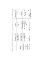
Table 8.2 Network delay specifications for voice applications
(ITU-T, G114)
Range (ms) Description
0–150 Acceptable for most services and
applications by users
150–400 Acceptable provided that administrators
are aware of the transmission time and
its impact on the transmission quality of
user applications
>400 Unacceptable for general network
planning purposes, however, only some
exceptional cases exceed this limit
the communications channel (in this case the Internet). Excessive delays will mean that
this ability is severely restricted. Variations in this delay (jitter) can possibly insert pauses
or even break up words making the voice communication unintelligible. This is why most
packetised voice applications use UDP to avoid recovering any packet loss or error.
The ITU-T considers network delay for voice applications in Recommendation G.114.
This recommendation defines three bands of one-way delay as shown in Table 8.2.
8.4.6 On-off model for voice traffic
It has been widely accepted that modelling packet voice can be conveniently based on
mimicking the characteristics of conversation – the alternating active and silent periods.
A two-phase on-off process can represent a single packetised voice source. Measurements
indicate that the average active interval is 0.352 s in length while the average silent interval
is 0.650 s. An important characteristic of a voice source to capture is the distribution of these
intervals. A reasonable good approximation for the distribution of the active interval is an
exponential distribution; however, this distribution does not represent the silent interval well.
Nevertheless, it often assumes that both these intervals are exponentially distributed when
modelling voice sources. The duration of voice calls (call holding time) and inter-arrival
time between the calls can be characterised using telephony traffic models.
During the active (on) interval, voice generates fixed size packets with a fixed inter-packet

spacing. This is the nature of voice encoders with fixed bit rate and fixed packetisation delay.
This packet generation process follows a Poisson process with exponentially distributed
inter-arrival times of mean T second or packet per second (pps) 1/T . As mentioned above,
both the on and off intervals are exponentially distributed, giving rise to a two-state MMPP
model. No packets are generated during the silent (off) interval. Figure 8.4 represents a
single voice source.
The mean on period is 1/ while the mean off period is 1/. The mean packet inter-
arrival time is T s. A superposition of N such voice sources results in the following N -state
birth–death model, Figure 8.5, where a state represents the number of sources in the on state.
This approach can model different voice codecs, with varying mean opinion score (MOS).
MOS isasystemofgrading the voice qualityoftelephoneconnections. Awiderange of listeners
Next Generation Internet (NGI) over Satellite 309
Poisson distribution with
average 1/T packets/s
α
λ
On Off
Figure 8.4 A single voice source, represented by a two-state MMPP
Nα2αα (N–1)α
(N-1)λ 2λλNλ
01
N
N – 1
……
pps
T
1
T
N – 1
T

N
Figure 8.5 Superposition of N voice sources with exponentially distributed inter-arrivals
judges the quality of a voice sample on a scale of one (bad) to five (excellent). The scores are
averaged to providethe MOS for the codec.The respective scores are 4.1(G.711), 3.92 (G.729)
and 3.8 (G.726). The parameters for this model are given in Table 8.2 with the additional
parameter representing packet inter-arrival time calculated using the following formula:
Inter_arrival_time =
1
average_traffic_sent_pps
(8.7)
where
average_traffic_sent =
codec_bit_rate
payload_size_bits
(8.8)
The mean off interval is typically 650 ms while the mean on interval is 350 ms.
8.4.7 Video traffic modelling
An emerging service of future multi-service networks is packet video communication. Packet
video communication refers to the transmission of digitised and packetised video signals in
real time. The recent development in video compression standards, such as ITU-T H.261,
ITU-T H.263, ISO MPEG-1, MPEG-2 and MPEG-4 [ISO99], has made it feasible to transport
video over computer communication networks. Video images are represented by a series
of frames in which the motion of the scene is reflected in small changes in sequentially
displayed frames. Frames are displayed at the terminal at some constant rate (e.g. 30 frames/s)
enabling the human eye to integrate the differences within the frame into a moving scene.
310 Satellite Networking: Principles and Protocols
In terms of the amount of bandwidth consumed, video streaming is high on the list.
Uncompressed, a one-second worth of video footage with a 300 ×200 pixels resolution
at a playback rate of 30 frames per second would require 1.8 byte/s. Apart from the high
throughput requirements, video applications also put a stringent requirement in terms of loss

and delay.
There are several factors affecting the nature of video traffic. Among these are compression
techniques, coding time (on- or off-line), adaptiveness of the video application, supported
level of interactivity and the target quality (constant or variable). The output bit rate of
the video encoder can either be controlled to produce a constant bit-rate stream which can
significantly vary the quality of the video (CBR encoding), or left uncontrolled to produce
a more variable bit-rate stream for a more fixed quality video (VBR encoding). Variable
bit-rate encoded video is expected to become a significant source of network traffic because
of its advantages in statistical multiplexing gains and consistent video quality.
Statistical properties of a video stream are quite different from that of voice or data. An
important property of video is the correlation structure between successive frames. Depending
on the type of video codecs, video images exhibit the following correlation components:
•
Line correlation is defined as the level of correlation between data at one part of the image
with data at the same part of the next line; also called spatial correlation.
•
Frame correlation is defined as the level of correlation between data at one part of the
image with data at the same part of the next image; also called temporal correlation.
•
Scene correlation is defined as the level of correlation between sequences of scenes.
Because of this correlation structure, it is no longer sufficient to capture the burst of video
sources. Several other measurements are required to characterise video sources as accurately
as possible. These measurements include:
•
Autocorrelation function: measures the temporal variations.
•
Coefficient of variation: measures the multiplexing characteristics when variable rate
signals are statistically multiplexed.
•
Bit-rate distribution: indicates together with the average bit rate and the variance, an

approximate requirement for the capacity.
As mentioned previously, VBR encoded video source is expected to be the dominant video
traffic source in the Internet. There are several statistical VBR source models. The models
are grouped into four categories – auto-regressive (AR)/Markov-based models, transform
expand sample (TES), self-similar and analytical/IID. These models were developed based
on several attributes of the actual video source. For instance, a video conferencing session,
which is based on the H.261 standards, would have very little scene changes and it is
recommended to use the dynamic AR (DAR) model. To model numerous scene changes
(as in MPEG-coded movie sequences), Markov-based models or self-similar models can be
used. The choice of which one to use is based on the number of parameters needed by the
model and the computational complexity involved. Self-similar models only require a single
parameter (Hurst or H parameter) but their computational complexity in generating samples
is high (because each sample is calculated from all previous samples). Markov chain models
on the other hand, require many parameters (in the form of transitional probabilities to model
Next Generation Internet (NGI) over Satellite 311
the scene changes), which again increase the computational complexity because it requires
many calculations to generate a sample.
8.4.8 Multi-layer modelling for internet WWW traffic
The Internet operations consist of a chain of interactions between the users, applications,
protocols and the network. This structured mechanism can be attributed to the layered
architecture employed in the Internet – a layering methodology was used in designing the
Internet protocol stack. Hence, it is only natural to try to model Internet traffic by taking
into account the different effects each layer of the protocol stack has on the resulting traffic.
The multi-layer modelling approach attempts to replicate the packet generation mechanism
as activated by the human users of the Internet and the Internet applications themselves.
In a multi-layer approach, packets are generated in a hierarchical process. It starts with
a human user arriving at a terminal and starting one or more Internet applications. This
action of invoking an application will start the chain of a succession of interactions between
the application and the underlying protocols on the source terminal and the corresponding
protocols and application on the destination terminal, culminating in the generation of packets

to be transported over the network. These interactions can generally be seen as ‘sessions’;
the definition of a session is dependent on the application generating it, as we will see later
when applying this method in modelling the WWW application. An application generates
at least one, but usually more, sessions. Each session comprises one or more ‘flows’; each
flow in turn comprises packets. Therefore, there are three layers or levels encountered in
this multi-layer modelling approach – session, flow and packet levels.
Take a scenario where a user arrives at a terminal and starts a WWW application by
launching a web browser. The user then clicks on a web link (or types in the web address)
to access the web sites of interest. This action generates what we call HTTP sessions.
The session is defined as the downloading of web pages from the same web server over
a limited period; this does not discount the fact that other definitions of a session are also
possible. The sessions in turn generate flows. Each flow is a succession of packets carrying
the information pertaining to a particular web page and packets are generated within flows.
This hierarchical process is depicted in Figure 8.6.
Browser launched Browser exited
Sessions
Flows
Packets
Parameters
Session arrival rate
Flow arrival rate
No. of flow/session
Packet arrival rate
No. of packet/session
Figure 8.6 Multi-layer modelling
312 Satellite Networking: Principles and Protocols
Depicted in the diagram are the suggested parameters for this model. More complex
models attempting to capture the self-similarity of web traffic might include the use of
heavy-tailed distributions to model any of the said parameters. Additional parameters such
as user think time and packet sizes are also modelled by heavy-tailed distributions. While

this type of model might be more accurate in capturing the characteristics of web traffic, it
comes with the added parameters and complexity.
8.5 Traffic engineering
A dilemma emerges for carriers and network operators: the cost to upgrade the infrastructure
as it is nowadays for fixed and mobile telephone networks, is too high to be supported
by revenues coming from Internet services. Actually, revenues coming from voice-based
services are quite high with respect to the ones derived by current Internet services. Therefore,
to obtain cost effectiveness it is necessary to design networks that make an effective use of
bandwidth or, in a broader sense, of network resources.
Traffic engineering (TE) is a solution that enables the fulfilment of all those requirements,
since it allows network resources to be used when necessary, where necessary and for the
desired amount of time. TE can be regarded as the ability of the network to control traffic
flows dynamically in order to prevent congestion, to optimise the availability of resources,
to choose routes for traffic flows while taking into account traffic loads and network state,
to move traffic flows towards less congested paths, to react to traffic changes or failures
timely.
The Internet has seen such a tremendous growth in the past few years. This growth has
correspondingly increased the requirements for network reliability, efficiency and service
quality. In order for the Internet service providers to meet these requirements, they need to
examine every aspect of their operational environment critically, assessing the opportunities
to scale their networks and optimise performance. However, this is not a trivial task. The
main problem is with the simple building block on which the Internet was built – namely
IP routing based on the destination address and simple metrics like hop count or link cost.
While this simplicity allows IP routing to scale to very large networks, it does not always
make good use of network resources. Traffic engineering (TE) has thus emerged as a major
consideration in the design and operation of large public Internet backbone networks. While
its beginnings can be traced back to the development of the public switched telephone
networks (PSTN), TE is fast finding a more crucial role to play in the design and operation
of the Internet.
8.5.1 Traffic engineering principles

Traffic engineering is ‘concerned with the performance optimisation of networks’. It seeks
to address the problem of efficient allocation of network resources to meet user constraints
and to maximise service provider benefit. The main goal of TE is to balance service and
cost. The most important task is to calculate the right amount of resources; too much and
the cost will be excessive, too little will result in loss of business or lower productivity.
As this service/cost balance is sensitive to the changes in business conditions, TE is thus a
continuous process to maintain an optimum balance.
Next Generation Internet (NGI) over Satellite 313
TE is a framework of processes whereby a network’s response to traffic demand (in terms
of user constraints such as delay, throughput and reliability) and other stimuli such as failure
can be efficiently controlled. Its main objective is to ensure the network is able to support as
much traffic as possible at their required level of quality and to do so by optimally utilising
its (the network’s) shared resources while minimising the costs associated with providing the
service. To do this requires efficient control and management of the traffic. This framework
encompasses:
•
traffic management through control of routing functions and QoS management;
•
capacity management through network control;
•
network planning.
Traffic management ensures that network performance is maximised under all conditions
including load shifts and failures (both node and link failures). Capacity management ensures
that the network is designed and provisioned to meet performance objectives for network
demands at minimum cost. Network planning ensures that the node and transport capacity
is planned and deployed in advance of forecasted traffic growth. These functions form an
interacting feedback loop around the network as shown in Figure 8.7.
The network (or system) shown in the figure is driven by a noisy traffic load (or signal)
comprising predictable average demand components added to unknown forecast errors and
load variation components. The load variation components have different time constants

ranging from instantaneous variations, hour-to-hour variations, day-to-day variations and
week-to-week or seasonal variations. Accordingly, the time constants of the feedback controls
are matched to the load variations and function to regulate the service provided by the
network through routing and capacity adjustments. Routing control typically applies on
minutes, days or possibly real-time time scales while capacity and topology changes are
much longer term (months to a year).
Advancement in optical switching and transmission systems enables ever-increasing
amounts of available bandwidth. The effect is that the marginal cost (i.e. the cost associated
with producing one additional unit of output) of bandwidth is rapidly being reduced: band-
width is getting cheaper. The widespread deployment of such technologies is accelerating
and network providers are now able to sell high-bandwidth transnational and international
Actual
load
Traffic
data
TE functions
• Traffic management
• Capacity management
• Network planning
Load
(+ uncertainties)
Forecasted
load
Routing control
Routing updates due to:
• Capacity changes
• Topology changes
Network
Figure 8.7 The traffic engineering process model
314 Satellite Networking: Principles and Protocols

connectivity simply by overprovisioning their networks. Logically, it would seem that in
the face of such developments and the abundance of available bandwidth, the need for TE
would be invalidated. On the contrary, TE still maintains its importance due principally to
the fact that both the number of users and their expectations are exponentially increasing in
parallel to the exponential increase in available bandwidth. A corollary of Moore’s law says,
‘As you increase the capacity of any system to accommodate user demand, user demand
will increase to consume system capacity’. Companies that have invested in such overpro-
visioned networks will want to recoup their investments. Service differentiation charging
and usage-proportional pricing are mechanisms widely accepted for doing so. To implement
these mechanisms, simple and cost-effective mechanisms for monitoring usage and ensuring
customers are receiving what they are requesting are required to make usage-proportional
pricing practical. Another important function of TE is to map traffic onto the physical infras-
tructure to utilise resources optimally and to achieve good network performance. Hence, TE
still performs a useful function for both network operators and customers.
8.5.2 Internet traffic engineering
Internet TE is defined as that aspect of Internet network engineering dealing with the issue of
performance evaluation and performance optimisation of operational IP networks. Internet
TE encompasses the application of technology and scientific principles to the measurement,
characterisation, modelling and control of Internet traffic. One of the main goals of Internet
TE is to enhance the performance of an operational network, both in terms of traffic-
handling capability and resource utilisation. Traffic-handling capability implies that IP traffic
is transported through the network in the most efficient, reliable and expeditious manner
possible. Network resources should be utilised efficiently and optimally while meeting the
performance objectives (delay, delay variation, packet loss and throughput) of the traffic.
There are several functions contributing directly to this goal. One of them is the control and
optimisation of the routing function, to steer traffic through the network in the most effective
way. Another important function is to facilitate reliable network operations. Mechanisms
should be provided that enhance network integrity and by embracing policies emphasising
network survivability. This results in a minimisation of the vulnerability of the network to
service outages arising from errors, faults and failures occurring within the infrastructure.

Effective TE is difficult to achieve in public IP networks due to the limited functional
capabilities of conventional IP technologies. One of the major problems lies in mapping
traffic flows onto the physical topology. In the Internet, mapping of flows onto a physical
topology was heavily influenced by the routing protocols used. Traffic flows simply followed
the shortest path calculated by interior gateway protocols (IGP) used within autonomous
systems (AS) such as open shortest path first (OSPF) or intermediate system – intermediate
system (IS-IS) and exterior gateway protocols (EGP) used to interconnect ASs such as border
gateway protocol 4 (BGP-4). These protocols are topology-driven and employ per-packet
control. Each router makes independent routing decisions based on the information in the
packet headers. By matching this information to a corresponding entry of a local instantiation
of a synchronised routing area link state database, the next hop or route for the packet is
then determined. This determination is based on shortest path computations (often equated
to lowest cost) using simple additive link metrics.
Next Generation Internet (NGI) over Satellite 315
While this approach is highly distributed and scalable, there is a major flaw – it does
not consider the characteristics of the offered traffic and network capacity constraints when
determining the routes. The routing algorithm tends to route traffic onto the same links and
interfaces, significantly contributing to congestion and unbalanced networks. This results
in parts of the network becoming over-utilised while other resources along alternate paths
remain under-utilised. This condition is commonly referred to as hyper aggregation. While
it is possible to adjust the value of the metrics used in calculating the IGP routes, it soon
became too complicated as the Internet core grows. Continuously adjusting the metrics also
adds instability to the network. Hence, congested parts are often resolved by adding more
bandwidth (overprovisioning), which is not treating the actual symptom of the problem in
the first place resulting in poor resource allocation or traffic mapping.
The requirements for Internet TE is not that much different than that of telephony net-
works – to have a precise control over the routing function in order to achieve specific
performance objectives both in terms of traffic-related performance and resource-related per-
formance (resource optimisation). However, the environment in which Internet TE is applied
is much more challenging due to the nature of the traffic and the operating environment of

the Internet itself. Traffic on the Internet is becoming more multi-class (compared to fixed
64 kbit/s voice in telephony networks) with different service requirements but contending
for the same network resources. In this environment, TE needs to establish resource-sharing
parameters to give preferential treatment to some service classes in accordance with a utility
model. The characteristics of the traffic are also proving to be a challenge – it exhibits
very dynamic behaviour, which is still to be understood and tends to be highly asymmet-
ric. The operating environment of the Internet is also an issue. Resources are augmented
constantly and they fail on a regular basis. Routing of traffic, especially when traversing
autonomous system boundaries, makes it difficult to correlate network topology with the
traffic flow. This makes it difficult to estimate the traffic matrix, the basic dataset needed
for TE.
An initial attempt at circumventing some of the limitations of IP with respect to TE was
the introduction of a secondary technology with virtual circuits and traffic management
capabilities (such as ATM) into the IP infrastructure. This is the overlay approach that
it consists of ATM switches at the core of the network surrounded by IP routers at the
edges. The routers are logically interconnected using ATM PVC, usually in a fully meshed
configuration. This approach allows virtual topologies to be defined and superimposed onto
the physical network topology. By collecting statistics on the PVC, a rudimentary traffic
matrix can be built. Overloaded links can be relieved by redirecting traffic to under-utilised
links.
ATM was used mainly because of its superior switching performance compared to IP
routing at that time (there are currently IP routers that are as fast if not faster than an
ATM switch). ATM also afforded QoS and TE capabilities. However, there are fundamental
drawbacks to this approach. Firstly, two networks of dissimilar technologies need to be
built and managed, adding to the increased complexity of network architecture and design.
Reliability concerns also increase because the number of network elements existing in a
routed path increases. Scalability is another issue especially in a fully meshed configuration
whereby the addition of another edge router would increase the number of PVC required
by nn −1/2, where n is the number of nodes (the ‘n-squared’ problem). There is also
the possibility of IP routing instability caused by multiple PVC failures following single

316 Satellite Networking: Principles and Protocols
link impairment in the ATM core. Concerning ATM itself, segmentation and reassembly
(SAR) is difficult to perform at high speeds. SAR is required because of the difference in
packet formats between IP and ATM – ATM is cell-based with a fixed size of 53 bytes. IP
packets would need to be segmented into ATM cells at the ingress of an ATM network. At
the egress, the cells would need to be reassembled into packets. Because of cell interleave,
SAR must perform queuing and scheduling for a large number of VCs. Implementing this at
STM-32 (10 Gbit/s) or higher speed is a very difficult task. Finally, the well-known problem
of ATM cell tax – the overhead penalty with the use of ATM, which is approximately
20% of the link bandwidth (e.g. 498 Mbit/s is wasted on ATM cell overhead on an STM-
16 or 2.4Gbit/s link,). Hence, there is a need to move away from the overlay model
to a more integrated solution. This was one of the motivations for the development of
MPLS.
8.6 Multi-protocol label switching (MPLS)
To improve on the best-effort service provided by the IP network layer protocol, new mech-
anisms such as differentiated services (Diffserv) and integrated services (Intserv), have been
developed to support QoS. In the Diffserv architecture, services are given different prior-
ities and resource allocations to support various types of QoS. In the Intserv architecture,
resources have to be reserved for individual services. However, resource reservation for indi-
vidual services does not scale well in large networks, since a large number of services have
to be supported, each maintaining its own state information in the network’s routers. Flow-
based techniques such as multi-protocol label switching (MPLS) have also been developed
to combine layer 2 and layer 3 functions to support QoS requirements.
MPLS introduces a new connection-oriented paradigm, based on fixed-length labels. This
fixed-length label-switching concept is similar but not the same as that utilised by ATM.
Among the key motivation for its development was to provide a mechanism for the seamless
integration of IP and ATM. As discussed in the previous chapter, the occurrence of IP
and ATM co-existence is something that is unavoidable in the pursuit for end-to-end QoS
guarantees. However, the architectural differences between the two technologies prove to
be a stumbling block for their smooth interoperation. Overlay models have been proposed

as solutions but they do not provide the single operating paradigm, which would simplify
network management and improve operational efficiency. MPLS is a peer model technology.
Compared to the overlay model, a peer model integrates layer 2 switching with layer
3 routing, yielding a single network infrastructure. Network nodes would typically have
integrated routing and switching functions. This model also allows IP routing protocols to
set up ATM connections and do not require address resolution protocols. While MPLS has
successfully merged the benefits of both IP and ATM, another application area in which
MPLS is fast establishing its usefulness is traffic engineering (TE). This also addresses other
major network evolution problems – throughput and scalability.
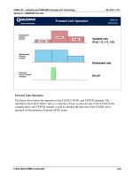
8.6.1 MPLS forwarding paradigm
MPLS is a technology that combines layer 2 switching technologies with layer 3 routing tech-
nologies. The primary objective of this new technology is to create a flexible networking fab-
Next Generation Internet (NGI) over Satellite 317
ric that provides increased performance and scalability. This includes TE capabilities. MPLS
is designed to work with a variety of transport mechanisms; however, initial deployment
will focus on leveraging ATM and frame relay, which are already deployed in large-scale
providers’ networks.
MPLS was initially designed in response to various inter-related problems with the cur-
rent IP infrastructure. These problems include scalability of IP networks to meet growing
demands, enabling differentiated levels of IP services to be provisioned, merging disparate
traffic types into a single network and improving operational efficiency in the face of tough
competition. Network equipment manufacturers were among the first to recognise these
problems and worked individually on their own proprietary solutions including tag switch-
ing, IP switching, aggregate route-based IP switching (ARIS) and cell switch router (CSR).
MPLS draws on these implementations in an effort to produce a widely applicable standard.
Because the concepts of forwarding, switching and routing are fundamental in MPLS, a
concise definition of each one of them is given below:
•
Forwarding is the process of receiving a packet on an input port and sending it out on an
output port.

•
Switching is forwarding process following the choosen path based information or knowl-
edge of current network resources and loading conditions. Switching operates on layer 2
header information.
•
Routing is the process of setting routes to understand the next hop a packet should
take towards its destination within and between networks. It operates on layer 3 header
information.
The conventional IP forwarding mechanism (layer 3 routing) is based on the source–
destination address pair gleaned from a packet’s header as the packet enters an IP network
via a router. The router analyses this information and runs a routing algorithm. The router
will then choose the next hop for the packet based on the results of the algorithm calculations
(which are usually based on the shortest path to the next router). More importantly, this
full packet header analysis must be performed on a hop-by-hop basis, i.e. at each router
traversed by the packet. Clearly, the IP packet forwarding paradigm is closely coupled to
the processor-intensive routing procedure.
While the efficiency and simplicity of IP routing is widely acknowledged, there are a
number of issues brought about by large routed networks. One of the main issues is the
use of software components to realise the routing function. This adds latency to the packet.
Higher speed, hardware-based routers are being designed and deployed, but these come at a
cost, which could easily escalate for large service providers’ or enterprise networks. There is
also difficulty in predicting the performance of a large meshed network based on traditional
routing concepts.
Layer 2 switching technologies such as ATM and frame relay utilise a different forwarding
mechanism, which is essentially based on a label-swapping algorithm. This is a much
simpler mechanism and can readily be implemented in hardware, making this approach
much faster and yielding a better price/performance advantage when compared to IP routing.
ATM is also a connection-oriented technology, between any two points, traffic flows along
a predetermined path are established prior to the traffic being submitted to the network.
Connection-oriented technology makes a network more predictable and manageable.

318 Satellite Networking: Principles and Protocols
8.6.2 MPLS basic operation
MPLS tries to solve the problem of integrating the best features of layer 2 switching and
layer 3 routing by defining a new operating methodology for the network. MPLS separates
packet forwarding from routing, i.e. separating the data-forwarding plane from the control
plane. While the control plane still relies heavily on the underlying IP infrastructure to
disseminate routing updates, MPLS effectively creates a tunnel underneath the control plane
using packet tags called labels. The concept of a tunnel is the key because it means the
forwarding process is no more IP-based and classification at the entry point of an MPLS
network is not relegated to IP-only information. The functional components of this solution
are shown in Figure 8.8, which do not differ much from the traditional IP router architecture.
The key concept of MPLS is to identify and mark IP packets with labels. A label is a short,
fixed-length, unstructured identifier that can be used to assist in the forwarding process.
Labels are analogous to the VPI/VCI used in an ATM network. Labels are normally local to
a single data link, between adjacent routers and have no global significance (as would an IP
address). A modified router or switch will then use the label to forward/switch the packets
through the network. This modified switch/router termed label switching router (LSR) is a
key component within an MPLS network. LSR is capable of understanding and participating
in both IP routing and layer 2 switching. By combining these technologies into a single
integrated operating environment, MPLS avoids the problem associated with maintaining
two distinct operating paradigms.
Label switching utilised in MPLS is based on the so-called MPLS shim header inserted
between the layer 2 header and the IP header. The structure of this MPLS shim header is
shown in Figure 8.9. Note that there can be several shim headers inserted between the layer
2 and IP headers. This multiple label insertion is called label stacking, allowing MPLS to
utilise a network hierarchy, provide virtual private network (VPN) services (via tunnelling)
and support multiple protocols [RFC3032].
Routing
updates
Routing

updates
Switch fabric
Control
component
Forwarding table
Forwarding component
Packet foreword
processing
Line card
Packets in Packets out
Layer 3
Layer 2
Routing protocol
Line card
Routing table &
Routing function
Figure 8.8 Functional components of MPLS
Next Generation Internet (NGI) over Satellite 319
La
yer 2
header
MPLS shim
header
MPLS shim
header
IP header
Label (20 bits)
EXP
(3 bits)
S

(1 bit)
TTL
(8 bits)
EXP: Experimental functions
S: Level of stack indicator, 1 indicates the bottom of the stack
TTL: Time to live
Figure 8.9 MPLS shim header structure
The MPLS forwarding mechanism differs significantly from conventional hop-by-hop
routing. The LSR participates in IP routing to understand the network topology as seen from
the layer 3 perspective. This routing knowledge is then applied, together with the results of
analysing the IP header, to assign labels to packets entering the network. Viewed on an end-
to-end basis, these labels combine to define paths called label switched paths (LSP). LSP are
similar to VCs utilised by switching technologies. This similarity is reflected in the benefits
afforded in terms of network predictability and manageability. LSP also enable a layer 2
forwarding mechanism (label swapping) to be utilised. As mentioned earlier, label swapping
is readily implemented in hardware, allowing it to operate at typically higher speeds than
routing. To control the path of LSP effectively, each LSP can be assigned one or more
attributes (see Table 8.3). These attributes will be considered in computing the path for the
LSP. There are two ways to set up an LSP – control-driven (i.e. hop-by-hop) and explicitly
Table 8.3 LSP attributes
Attribute name Meaning of attribute
Bandwidth The minimum requirement on the reserverable bandwidth for the LSP to
be set up along that path
Path attribute An attribute that decides whether the path for the LSP should be
manually specified or dynamically computed by constraint-based routing
Setup priority The attribute that decides which LSP will get the resource when multiple
LSPs compete for it
Holding priority The attribute that decides whether an established LSP should be
pre-empted by a new LSP
Affinity An administratively specified property of an LSP to achieve some

desired LSP placement
Adaptability Whether to switch the LSP to a more optimal path when one becomes
available
Resilience The attribute that decides to re-route the LSP when the current path fails
320 Satellite Networking: Principles and Protocols
routed LSP (ER-LSP). Since the overhead of manually configuring LSP is very high, there
is a need on service providers’ behalf to automate the process by using signalling protocols.
These signalling protocols distribute labels and establish the LSP forwarding state in the
network nodes. A label distribution protocol (LDP) is used to set up a control-driven LSP
while RSVP-TE and CR-LDP are the two signalling protocols used for setting up ER-LSP.
The label swapping algorithm is a more efficient form of packet forwarding, compared
to the longest address match-forwarding algorithm used in conventional layer 3 routing.
The label-swapping algorithm requires packet classification at the point of entry into the
network from the ingress label edge router (LER) to assign an initial label to each packet.
Labels are bound to forwarding equivalent classes (FEC). An FEC is defined as a group
of packets that can be treated in an equivalent manner for purposes of forwarding (share
the same requirements for their transport). The definition of FEC can be quite general.
FEC can relate to service requirements for a given set of packets or simply on source and
destination address prefixes. All packets in such a group get the same treatment en route to
the destination. In a conventional packet forwarding mechanism, FEC represent groups of
packets with the same destination address; then the FEC should have their respective next
hops. However, it is the intermediate nodes processing the FEC grouping and mapping. As
opposed to conventional IP forwarding, in MPLS, it is the edge-to-edge router assigning
packets to a particular FEC when the packet enters the network. Each LSR then builds a
table to specify how to forward packets. This forwarding table, called a label information
base (LIB), comprises FEC-to-label bindings.
In the core of the network, LSR ignore the header of network layer packets and simply
forward the packet using the label with the label-swapping algorithm. When a labelled packet
arrives at a switch, the forwarding component uses the pairing, input port number/incoming
interface, incoming label value, to perform an exact match search of its forwarding table.

When a match is found, the forwarding component retrieves the pairing, output port num-
ber/outgoing interface, outgoing label value, and the next-hop address from the forwarding
table. The forwarding component then replaces the incoming label with the outgoing label
and directs the packet to the outbound interface for transmission to the next hop in the LSP.
When the labelled packet arrives at the egress LER (point of exit from the network), the
forwarding component searches its forwarding table. If the next hop is not a label switch, the
egress LSR discards (pop-off) the label and forwards the packet using conventional longest
match IP forwarding. Figure 8.10 shows the label swapping process.
• Perform Layer 3 lookup.
• Map to FEC.
• Attach label and forward
out appropriate interface
according to FEC.
• Perform exact match on
incoming label.
• Lookup outgoing interface
and label.
• Swap labels and forward
out appropriate interface.
• Pop-off label.
• Perform Layer 3
lookup.
• Forward according
to Layer 3 lookup.
Ingress LER
A
Interior LSR
B
Egress LER
C

IP packet
IP packet
Label
Host
Z
IP packet
Label
IP packet
Figure 8.10 Label swapping and forwarding process
Next Generation Internet (NGI) over Satellite 321
LSP can also allow minimising the number of hops, to meet certain bandwidth require-
ments, to support precise performance requirements, to bypass potential points of congestion,
to direct traffic away from the default path, or simply to force traffic across certain links
or nodes in the network. Label swapping gives a huge flexibility in the way that it assigns
packets to FEC. This is because the label swapping forwarding algorithm is able to take
any type of user traffic, associate it with an FEC, and map the FEC to an LSP that has
been specifically designed to satisfy the FEC requirements; therefore allowing a high level
of control in the network. These are the features, which lend credibility to MPLS to support
traffic engineering (TE). We will discuss further the application of MPLS in TE in a later
section.
8.6.3 MPLS and Diffserv interworking
The introduction of a QoS enabled protocol into a network supporting various other QoS
protocols would undoubtedly lead to the requirement for these protocols to interwork with
each other in a seamless fashion. This requirement is essential to the QoS guarantees to the
packets traversing the network. It is an important issue of interworking MPLS with Diffserv
and ATM.
The combination of MPLS and Diffserv provides a scheme, which is mutually beneficial
for both. Path-oriented MPLS can provide Diffserv with a potentially faster and more
predictable path protection and restoration capabilities in the face of topology changes, as
compared to conventional hop-by-hop routed IP networks. Diffserv, on the other hand, can

act as QoS architecture for MPLS. Combined, MPLS and Diffserv can provide the flexibility
to provide different treatments to certain QoS classes requiring path protection.
IETF3270 specifies a solution for supporting Diffserv behaviour aggregates (BA) and
their corresponding per hop behaviours (PHB) over an MPLS network. The key issue for
supporting Diffserv over MPLS is how to map Diffserv to MPLS. This is because LSR
cannot see an IP packet’s header and the associated DSCP values, which links the packet
to its BA and consequently to its PHB, as PHB determines the scheduling treatment and, in
some cases, the drop probability of a packet. LSR only look for labels, read their contents
and decide the next hop. For an MPLS domain to handle a Diffserv packet appropriately,
the labels must contain some information regarding the treatment on the packet.
The solution to this problem is to map the six-bit DSCP values to the three-bit EXP field
of the MPLS shim header. This solution relies on the combined use of two types of LSP:
•
A LSP that can transport multiple ordered aggregates, so that the EXP field of the MPLS
shim header conveys to the LSR with the PHB applied to the packet (covering both
information about the packet’s scheduling treatment and its drop precedence). An ordered
aggregate (OA) is a set of BAs sharing an ordering constraint. Such an LSP refers to as
EXP-Inferred-PSC-LSP (E-LSP), when defining PSC as a PHB scheduling class. The set
of one or more PHB applies to the BAs belonging to a given OA. With this method, it
can map up to eight DSCPs to a single E-LSP.
•
A LSP that can transport only a single ordered aggregate, so that the LSR exclusively infer
the packet scheduling treatment exclusively from the packet label value. The packet drop
precedence is conveyed in the EXP field of the MPLS shim header or in the encapsulating
link layer specific selective drop mechanism, where in such cases the MPLS shim header
322 Satellite Networking: Principles and Protocols
is not used (e.g. MPLS over ATM). Such LSP refer to label-only-inferred-PSC-LSP
(L-LSP). With this method, an individual L-LSP has a dedicated Diffserv code point.
8.6.4 MPLS and ATM interworking
MPLS and ATM can interwork at network edges to support and bring multiple services

into the network core of an MPLS domain. In this instance, ATM connections need to be
transparent across the MPLS domain over MPLS LSP. Transparency in this context means
that ATM-based services should be carried over the domain unaffected.
There are several requirements that need to be addressed concerning MPLS and ATM
interworking. Some of these requirements are:
•
The ability to multiplex multiple ATM connections (VPC and/or VCC) into an MPLS
LSP.
•
Support for the traffic contracts and QoS commitments made to the ATM connections.
•
The ability to carry all the AAL types transparently.
•
Transport of RM cells and CLP information from the ATM cell header.
Transport of ATM traffic over the MPLS uses only the two-level LSP stack. The two-level
stack specifies two types of LSP. A transport LSP (T-LSP) transports traffic between two
ATM-MPLS interworking devices located at the boundaries of the ATM-MPLS networks.
This traffic can consist of a number of ATM connections, each associated with an ATM
service category. The outer label of the stack (known as a transport label) defines a T-LSP,
i.e. the S field of the shim header is set to 0 to indicate it is not the bottom of the stack. The
second type of LSP is an interworking LSP (I-LSP), nested within the T-LSP (identified by
an interworking label), which carries traffic associated with a particular ATM connection, i.e.
one I-LSP is used for an ATM connection. I-LSP also provides support for VP/VC switching
functions. One T-LSP may carry more than one I-LSP. Because an ATM connection is
bi-directional while an LSP is unidirectional, two different I-LSPs, one for each direction
of the ATM connection, are required to support a single ATM connection. Figure 8.11
shows the relationship between T-LSP, I-LSP and ATM connections. The interworking unit
(IWU) encapsulates ATM cells in the ATM-to-MPLS direction, into a MPLS frame. For the
MPLS-to-ATM direction, the IWU reconstructs the ATM cells.
With regarding to support of ATM traffic contracts and QoS commitments to ATM

connections, the mapping of ATM connections to I-LSP and subsequently to T-LSP must
take into consideration the TE properties of the LSP. There are two methods to implement
this.
Firstly, a single T-LSP can multiplex all the I-LSP associated to several ATM connections
with different service categories. This type of LSP is termed class multiplexed LSP. It groups
the ATM service categories into groups and maps each group into a single LSP. As an
example for the second scenario, it groups the categories initially into real-time traffic (CBR
and rt-VBR) and non-real-time traffic (nrt-VBR, ABR, UBR). It transports the real-time
traffic over one T-LSP while the non-real-time traffic over another T-LSP. It can implement
class multiplexed LSP by using either L-LSP or E-LSP. Class multiplexed L-LSP must meet
the most stringent QoS requirements of the ATM connections transported by the LSP. This
is because L-LSP treats every packet going through it the same. Class multiplexed E-LSP, on
Next Generation Internet (NGI) over Satellite 323
(a)
ATM
network
ATM
network
MPLS
network
ATM VP/VC link
IWU
Transport LSP
Interworking LSP
ATM MPLS
IWU
MPLS ATM
(b)
Figure 8.11 ATM-MPLS networks interworking. (a) ATM-MPLS network interworking architecure.
(b) the relationship between transport LSP, interworking LSP and ATM link

the other hand, identifies the scheduling and dropping treatments applied to a packet based
on the value of the EXP field inside the T-LSP label. Each LSR can then apply different
scheduling treatments for each packet transported over the LSP. This method also requires
a mapping between ATM service categories and the EXP bits.
Secondly, an individual T-LSP is allocated to each ATM service class. This LSP is termed
class based LSP. There can be more than one connection per ATM service class. In this
case, the MPLS domain would search for a path that meets the requirement of one of the
connections.
8.6.5 MPLS with traffic engineering (MPLS-TE)
An MPLS domain still requires IGP such as OSPF and IS-IS to calculate routes through the
domain. Once it has computed a route, it uses signalling protocols to establish LSP along
the route. Traffic that satisfies a given FEC associated with a particular LSP is then sent
down the LSP.
The basic problem addressed by TE is the mapping of traffic onto routes to achieve
the performance objectives of the traffic while optimising the resources at the same time.
Conventional IGP such as open shortest path first (OSPF), makes use of pure destination
address-based forwarding. It selects routes based on simply the least cost metric (or shortest
path). Traffic from different routers therefore converge on this particular path, leaving the
other paths under-utilised. If the selected path becomes congested, there is no procedure to
off-load some of the traffic onto the alternative path.
For TE purposes, the LSR should build a TE database within the MPLS domain. This
database holds additional information regarding the state of a particular link. Additional
link attributes may include maximum link bandwidth, maximum reserverable bandwidth,
current bandwidth utilisation, current bandwidth reservation and link affinity or colour
(an administratively specified property of the link). These additional attributes are carried
324 Satellite Networking: Principles and Protocols
by TE extensions of existing IGP – OSPF-TE and IS-IS TE. This enhanced database will
then be used by the signalling protocols to establish ER-LSP.
The IETF has specified LDP as the signalling protocol for setting up LSP. LDP is usually
used for hop-by-hop LSP set up, whereby each LSR determines the next interface to route the

LSP based on its layer 3 routing topology database. This means that hop-by-hop LSP follow
the path that normal layer 3 routed packets will take. There are two signalling protocols:
RSVP-TE (RSVP with TE extension) and CR-LDP (constraint-based routing LDP) control
the LSP for TE applications. These protocols are used to establish traffic-engineered ER-
LSP. An explicit route specifies all the routers across the network with a precise sequence
of steps from ingress to egress. Packets must follow this route strictly. Explicit routing is
useful to force an LSP down a path that is different from the one offered by the routing
protocol. Explicit routing can also be used to distribute traffic in a busy network, to route
around failed or congestion hot spots, or to provide pre-allocated back-up LSP to protect
against network failures.
8.7 Internet protocol version 6 (IPv6)
Recently, there has been increasing interest in research, development and deployment in
IPv6. The protocol itself it very easy to understands. Like any new protocols and networks,
it faces a great challenge in compatibility with the existing operational networks, balancing
economic cost and benefit of the evolution towards IPv6, and smooth change over from IPv4
to IPv6. It is also a great leap. However, most of these are out of the scope of this book.
Here we only discuss the basics of IPv6 and issues on IPv6 networking over satellites.
8.7.1 Basics of internet protocol version 6 (IPv6)
The IP version 6 (IPv6), which the IETF have developed as a replacement for the current IPv4
protocol, incorporates support for a flow label within the packet header, which the network
can use to identify flows, much as VPI/VCI are used to identify streams of ATM cells.
RSVP helps to associate with each flow a flow specification (flow spec) that characterises
the traffic parameters of the flow, much as the ATM traffic contract is associated with an
ATM connection.
IPv6 can support integrated services with QoS with such mechanisms and the definition
of protocols like RSVP. It extends the IPv4 protocol to address the problems of the current
Internet to:
•
support more host addresses;
•

reduce the size of the routing table;
•
simplify the protocol to allow routers to process packets faster;
•
have better security (authentication and privacy);
•
provide QoS to different types of services including real-time data;
•
aid multicasting (allow scopes);
•
allow mobility (roam without changing address);
•
allow the protocol to evolve;
•
permit coexisting of old and new protocols.
Next Generation Internet (NGI) over Satellite 325
Flow label
Payload length Next header
0 8 16 24 (31)
Version
Hop limit
0 8 16 24
Priority
Source Address
Source Address
Source Address
Source Address
Destination Address
Destination Address
Destination Address

Destination Address
Figure 8.12 IPv6 packet header format
Compared to IPv4, IPv6 has made significant changes to the IPv4 packet format in order
to achieve the objectives of the next generation Internet with the network layer functions.
Figure 8.12 shows the IPv6 packet header format. The functions of its fields is summarised
as the following:
•
The version field has the same function as IPv4. It is 6 for IPv6 and 4 for IPv4.
•
The priority field identifies packets with different real-time delivery requirements.
•
The flow label field is used to allow source and destination to set up a pseudo-connection
with particular properties and requirements.
•
The payload field is the number of bytes following the 40-byte header, instead of total
length in IPv4.
•
The next header field tells which transport handler to pass the packet to, like the protocol
field in the IPv4.
•
The hop limit field is a counter used to limit packet lifetime to prevent the packet staying
in the network forever, like the time to live field in IPv4.
•
The source and destination addresses indicate the network number and host number, four
times larger than IPv4
•
There are also extension headers like the options in IPv4. Table 8.4 shows the IPv6
extension header.
Each extension header consists of next header field, and fields of type, length and value.
In IPv6, the optional features become mandatory features: security, mobility, multicast and

transitions. IPv6 tries to achieve an efficient and extensible IP datagram in that:
•
the IP header contains less fields that enable efficient routing and performance;
•
extensibility of header offers better options;
•
the flow label gives efficient processing of IP datagram.
326 Satellite Networking: Principles and Protocols
Table 8.4 IPv6 extension headers
Extension header Description
Hop-by-hop options Miscellaneous information for routers
Destination options Additional information for the destination
Routing Loose list of routers to visit
Fragmentation Management of datagram fragments
Authentication Verification of the sender’s identity
Encrypted security payload Information about the encrypted contents
8.7.2 IPv6 addressing
IPv6 has introduced a large addressing space to address the shortage of IPv4 addresses. It
uses 128 bits for addresses, four times the 32 bits of the current IPv4 address. It allows
about 34 ×10
38
possible addressable nodes, equivalent to 1030 addresses per person on the
planet. Therefore, we should never exhaust IPv6 addresses in the future Internet.
In IPv6, there is no hidden network and host. All hosts can be servers and are reachable
from outside. This is called global reachability. It supports end-to-end security, flexible
addressing and multiple levels of hierarchy in the address space.
It allows autoconfiguration, link-address encapsulation, plug & play, aggregation, multi-
homing and renumbering.
The address format is x:x:x:x:x:x:x:x, where x is a 16-bit hexadecimal field. For
example, herewith is an IPv6 address:

2001  FFFF  1234  0000  0000  C1C0  ABCD  8760
It is case sensitive and is different from the following address:
2001  FFFF  1234  0000  0000  c1c0:abcd
 8760
Leading zeros in a field are optional:
2001  0
 1234  0  0  C1C0  ABCD  8760
Successive fields of 0 can be written as ‘::’. For example:
2001  0  1234 C1C0  FFCD  8760
We can also rewrite the following addresses:
FF02  0  0  0  0  0  0  1 into FF02 1
0  0  0  0  0  0  0  1 into 1 and
0  0  0  0  0  0  0  0 into 
Next Generation Internet (NGI) over Satellite 327
But we can only use ‘::’ once in an address. An address like this is not valid:
2001 1234 C1C0  FFCD  8760
IPv6 addresses are also different in a URL. It only allows fully qualified domain names
(FQDN). An IPv6 address is enclosed in brackets such as http://[2001:1:4F3A::20F6:AE14]:
8080/index.html. Therefore, URL parsers have to be modified, and it could be a barrier for
users.
IPv6 address architecture defines different types of address: unicast, multicast and anycast.
There are also unspecified and loop back addresses. Unspecified addresses can be used as a
placeholder when no address is available, such as in an initial DHCP request and duplicate
address detection (DAD). Loop back addresses identify the node itself as the local host using
127.0.0.1 in IPv4 and 0:0:0:0:0:0:0:1 or simply ::1in IPv6. It can be used
for testing IPv6 stack availability, for example, ping6 : :1.
The scope of IPv6 addresses allows link-local and site-local. It allows aggregatable global
addresses including multicast and anycast, but there is no broadcast address in IPv6.
The link-local scoped address is new in IPv6: ‘scope = local link’ (i.e. WLAN, subnet).
It can only be used between nodes of the same link, but cannot be routed. It allows

autoconfiguration on each interface using a prefix plus interface identifier (based on MAC
address) in the format of ‘FE80:0:0:0:<interface identifier>’. It gives every node an IPv6
address for start-up communications.
The site-local scoped address has ‘scope = site (a network of links)’. It can only be used
between nodes of the same site, but cannot be routed outside the site, and is very similar to
IPv4 private addresses. There is no default configuration mechanism to assign it. It has the
format of ‘FEC0:0:0:<subnet id>:<interface id>’ where the <subnet id> has 16 bits capable
of addressing 64 k subnets. It can be used to number a site before connecting to the Internet
or for private addresses (e.g. local printers).
The aggregatable global address is for generic use and allows globally reach. The address
is allocated by IANA (Internet assigned number authority) with a hierarchy of tier-1 providers
as top-level aggregator (TLA), intermediate providers as next-level aggregator (NLA), and
finally sites and subnets at the bottom, as shown in Figure 8.13.
IPv6 support multicast, i.e. one-to-many communications. Multicast is used instead, mostly
on local links. The scope of the addresses can be node, link, site, organisation and global.
Unlike IPv4, it does not use time to live (TTL). IPv6 multicast addresses have a format
of ‘FF<flags><scope>::<multicast group>’. Any IPv6 node should recognise the following
addresses as identifying itself (see Table 8.5):
•
link-local address for each interface;
•
assigned (manually or automatically) unicast/anycast addresses;
TLA RES NLAs SLA Interface ID
48 bits 16 bits 64 bits
Figure 8.13 Structure of the aggregatable global address
328 Satellite Networking: Principles and Protocols
Table 8.5 Some reserved multicast addresses
Address Scope Use
FF01::1 Interface-local All nodes
FF02::1 Link-local All nodes

FF01::2 Interface-local All routers
FF02::2 Link-local All routers
FF05::2 Site-local All routers
FF02::1:FFXX:XXXX Link-local Solicited nodes
•
loop back address;
•
all-nodes multicast address;
•
solicited-node multicast address for each of its assigned unicast and anycast address;
•
multicast address of all other groups to which the host belongs.
The anycast address is one-to-nearest, which is great for discovery functions. Anycast
addresses are indistinguishable from unicast addresses, as they are allocated from the unicast
address space. Some anycast addresses are reserved for specific uses, for example, router-
subnet, mobile IPv6 home-agent discovery and DNS discovery. Table 8.6 shows the IPv6
address architecture.
Table 8.6 IPv6 addressing architecture
Prefix Hex Size Allocation
0000 0000 0000-00FF 1/256 Reserved
0000 0001 0100-01FF 1/256 Unassigned
0000 001 0200-03FF 1/128 NSAP
0000 010 0400-05FF 1/128 Unassigned
0000 011 0600-07FF 1/128 Unassigned
0000 1 0800-0FFF 1/32 Unassigned
0001 1000-1FFF 1/16 Unassigned
001 2000-3FFF 1/8 Aggregatable:
IANA to registry
010, 011, 100, 101, 110 4000-CFFF 5/8 Unassigned
1110 D000-EFFF 1/16 Unassigned

1111 0 F000-F7FF 1/32 Unassigned
1111 10 F800-FBFF 1/64 Unassigned
1111 110 FC00-FDFF 1/128 Unassigned
1111 1110 0 FE00-FE7F 1/512 Unassigned
1111 1110 10 F800-FEBF 1/1024 Link-local
1111 1110 11 FEC0-FEFF 1/1024 Site-local
1111 1111 FF00-FFFF 1/256 Multicast
Next Generation Internet (NGI) over Satellite 329
When a node has many IPv6 addresses, to select which one to use for the source and
destination addresses for a given communication, one should address the following issues:
•
scoped addresses are unreachable depending on the destination;
•
preferred vs. deprecated addresses;
•
IPv4 or IPv6 when DNS returns both;
•
IPv4 local scope (169.254/16) and IPv6 global scope;
•
IPv6 local scope and IPv4 global scope;
•
mobile IP addresses, temporary addresses, scope addresses, etc.
8.7.3 IPv6 networks over satellites
We have learnt through the book to treat the satellite networks as generic networks with
different characteristics and IP networks interworking with other different networking tech-
nologies. Therefore, all the concepts, principles and techniques can be applied to IPv6 over
satellites. Though IP has been designed for internetworking purposes, the implementation
and deployment of any new version or new type of protocol always face some problems.
These also have potential impacts on all the layers of protocols including trade-offs between
processing power, buffer space, bandwidth, complexity, implementation costs and human

factors. To be concise, we will only summarise the issues and scenarios on internetworking
between IPv4 and IPv6 as the following:
•
Satellite network is IPv6 enabled: this raises issues on user terminals and terrestrial IP
networks. We can imagine that it is not practical to upgrade them all at the same time.
Hence, one of the great challenges is how to evolve from current IP networking over
satellite towards the next generation network over satellites. Tunnelling from IPv4 to IPv6
or from IPv6 to IPv4 is inevitable, hence generating great overheads. Even if all networks
are IPv6 enabled, there is still a bandwidth efficiency problem due to the large overhead
of IPv6.
•
Satellite network is IPv4 enabled: this faces similar problems to the previous scenario,
however, satellite networks may be forced to evolve to IPv6 if all terrestrial networks and
terminals start to run IPv6. In terrestrial networks when bandwidth is plentiful, we can
afford to delay the evolution. In satellite networks, such a strategy may not be practical.
Hence, timing, stable IPv6 technologies and evolution strategies all play an important role.
8.7.4 IPv6 transitions
The transition of IPv6 towards next-generation networks is a very important aspect. Many
new technologies failed to succeed because of the lack of transition scenarios and tools. IPv6
was designed with transition in mind from the beginning. For end systems, it uses a dual
stack approach as show in Figure 8.14; and for network integration, it uses tunnels (some
sort of translation from IPv6-only networks to IPv4-only networks).
Figure 8.14 illustrates a node that has both IPv4 and IPv6 stacks and addresses. The IPv6-
enabled application requests both IPv4 and IPv6 destination addresses. The DNS resolver
returns IPv6, IPv4 or both addresses to the application. IPv6/IPv4 applications choose the
address and then can communicate with IPv4 nodes via IPv4 or with IPv6 nodes via IPv6.
330 Satellite Networking: Principles and Protocols
Data Link (e.g. Ethernet)
IPv4 IPv6
0x0800 0x86dd

TCP UDP
Applications
Figure 8.14 Illustration of dual stack host
8.7.5 IPv6 tunnelling through satellite networks
Tunnelling IPv6 in IPv4 is a technique use to encapsulate IPv6 packets into IPv4 packets
with protocol field 41 of the IP packet header (see Figure 8.15). Many topologies are possible
including router to router, host to router, and host to host. The tunnel endpoints take care of
the encapsulation. This process is ‘transparent’ to the intermediate nodes. Tunnelling is one
of the most vital transition mechanisms.
In the tunnelling technique, the tunnel endpoints are explicitly configured and they must be
dual stack nodes. If the IPv4 address is the endpoint for the tunnel, it requires reachable IPv4
addresses. Tunnel configuration implies manual configuration of the source and destination
IPv4 addresses and the source and destination IPv6 addresses. Tunnel configuration cases
can be between two hosts, one host and one router as shown in Figure 8.16, or two routers
of two IPv6 networks as shown in Figure 8.17.
8.7.6 The 6to4 translation via satellite networks
The 6to4 translation is a technique used to interconnect isolated IPv6 domains over an IPv4
network with automatic establishment of a tunnel. It avoids the explicit tunnels used in the
tunnelling technique by embedding the IPv4 destination address in the IPv6 address. It uses
the reserved prefix ‘2002::/16’ (2002::/16 ≡ 6to4). It gives the full 48 bits of the address to a
site based on its external IPv4 address. The IPv4 external address is embedded: 2002:<ipv4
ext address>::/48 with the format, ‘2002:<ipv4add>:<subnet>::/64’. Figures 8.18 and 8.19
show the tunnelling techniques.
Ethernet
0x0800
IPv4
41
IPv6
6
TCP

25
SMTP
Payload (Message)
Encapsulated IPv6 packet
Original IPv6 packet
Ethernet
0x86dd
IPv6
6
SMTP
Payload (Message)
TCP
25
Figure 8.15 Encapsulation of IPv6 packet into IPv4 packet
Next Generation Internet (NGI) over Satellite 331
Satellite as Access Network
IPv4 network
Router
IPv6 in IPv4
IPv6
IPv4 address: 192.168.1.1
IPv6 address: 3ffe:b00:a:1::1
src = 3ffe:b00:a:1::1
des
= 3ffe:b00:a:3::2
src = 3ffe:b00:a:1::1
des
= 3ffe:b00:a:3::2
IPv6 address:
3ffe:b00:a:3::2

IP address
v4: 192.168.2.1
v6: 3ffe:b00:a:1::2
IPv6 address
3ffe:b00:a:5::1
IPv6 headerPayload IPv6 headerPayload
src = 192.168.1.1
des
= 192.168.2.1
IPv6 headerPayload IPv4 header
Figure 8.16 Host to router tunnelling through satellite access network
Satellite as Access Network
IPv4 network
Router
IPv6 in IPv4
IPv6
IPv6 address:
3ffe:b00:a:1::1
src =3ffe:b00:a:1::1
des=3ffe:b00:a:3::2
src = 3ffe:b00:a:1::1
des
= 3ffe:b00:a:3::2
IPv6 address:
3ffe:b00:a:3::2
IPv4 address:
192.168.2.1
IPv6 header

Payload IPv6 headerPayload

src = 192.168.1.1
des
= 192.168.2.1
IPv6 headerPayload IPv4 header
Router
IPv6
IPv4 address:
192.168.1.1
Figure 8.17 Router to router tunnelling through satellite core network
Satellite as Access Network
IPv4 network
6to4
Router
IPv6 in IPv4
IPv6
IPv4 address: 192.168.1.1
IPv6 address: 2002:c0a8:101:1::1
src = 2002.c0a8:101:1::1
des
= 2002:c0a8:201:2::2
IPv6 address:
200:c0a8:101:1::1
IPv4 address
192.168.2.1
IPv6 headerPayload IPv6 headerPayload
src = 192.168.1.1
des
= 192.168.2.1
IPv6 headerPayload IPv4 header
src = 2002:c0a8:101:1::1

des
= 2002:c0a8:201:2::2
Figure 8.18
332 Satellite Networking: Principles and Protocols
Satellite as Access Network
IPv4 network
6to4
Router
IPv6 in IPv4
IPv6
IPv6 address:
2002:c0a8:101:1::1
src
= 2002:c0a8:101:1::1
des
= 2002:c0a8:201:2::2
IPv6 address:
2002:c0a8:201:2::2
IPv4 address:
192.168.2.1
IPv6 headerPayload IPv6 headerPayload
src = 192.168.1.1
des
= 192.168.2.1
IPv6 headerPayload IPv4 header
6to4
Router

IPv6
IPv4 address:

192.168.1.1
src = 2002:c0a8:101:1::1
des
= 2002:c0a8:201:2::2
Figure 8.19 The 6to4 translation via satellite core network
To support 6to4, the egress router implementing 6to4 must have a reachable external
IPv4 address. It is a dual-stack node. It is often configured using a loop back address.
Individual nodes do not need to support 6to4. The prefix 2002 may be received from router
advertisements. It does not need to be dual stack.
8.7.7 Issues with 6to4
IPv4 external address space is much smaller than IPv6 address space. If the egress router
changes its IPv4 address, then it means that the full IPv6 internal network needs to be
renumbered. There is only one entry point available. It is difficult to have multiple network
entry points to include redundancy.
Concerning application aspects of IPv6 transitions, there also other problems with IPv6 at
the application layer: the support of IPv6 in the operating systems (OS) and applications is
unrelated; dual stack does not mean having both IPv4 and IPv6 applications; DNS does not
indicate which IP version to be used; and it is difficult to support manyversions of applications.
Therefore, the application transitions of different cases can be summarised as the following
(also see Figure 8.20):
•
For IPv4 applications in a dual-stack node, the first priority is to port applications to IPv6.
•
For IPv6 applications in a dual-stack node, use IPv4-mapped IPv6 address ‘::FFFF:x.y.z.w’
to make IPv4 applications work in IPv6 dual stack.
•
For IPv4/IPv6 applications in a dual-stack node, it should have a protocol-independent API.
•
For IPv4/IPv6 applications in an IPv4-only node, it should be dealt with on a case-by-case
basis, depending on applications/OS support.

8.7.8 Future development of satellite networking
It is difficult to predict the future, sometime impossible, but it is not too difficult to predict
the trends towards future development if we have enough past and current knowledge. In
addition to integrating satellites into the global Internet infrastructure, one of the major tasks
is to create new services and applications to meet the needs of people. Figure 8.21 illustrates
an abstract vision of future satellite networking.