Theory and applications of ofdm and cdma wideband wireless communications phần 1 ppsx
Bạn đang xem bản rút gọn của tài liệu. Xem và tải ngay bản đầy đủ của tài liệu tại đây (832.4 KB, 43 trang )
TEAM LinG
Theory and Applications of
OFDM and CDMA
Theory and Applications of
OFDM and CDMA
Wideband Wireless Communications
Henrik Schulze
and
Christian L
¨
uders
Both of
Fachhochschule S¨udwestfalen
Meschede, Germany
Copyright 2005 John Wiley & Sons Ltd, The Atrium, Southern Gate, Chichester,
West Sussex PO19 8SQ, England
Telephone (+44) 1243 779777
Email (for orders and customer service enquiries):
Visit our Home Page on www.wiley.com
All Rights Reserved. No part of this publication may be reproduced, stored in a retrieval system or transmitted
in any form or by any means, electronic, mechanical, photocopying, recording, scanning or otherwise, except
under the terms of the Copyright, Designs and Patents Act 1988 or under the terms of a licence issued by the
Copyright Licensing Agency Ltd, 90 Tottenham Court Road, London W1T 4LP, UK, without the permission in
writing of the Publisher. Requests to the Publisher should be addressed to the Permissions Department, John
Wiley & Sons Ltd, The Atrium, Southern Gate, Chichester, West Sussex PO19 8SQ, England, or emailed to
, or faxed to (+44) 1243 770620.
Designations used by companies to distinguish their products are often claimed as trademarks. All brand names
and product names used in this book are trade names, service marks, trademarks or registered trademarks of
their respective owners. The Publisher is not associated with any product or vendor mentioned in this book.
This publication is designed to provide accurate and authoritative information in regard to the subject matter
covered. It is sold on the understanding that the Publisher is not engaged in rendering professional services. If
professional advice or other expert assistance is required, the services of a competent professional should be
sought.
Other Wiley Editorial Offices
John Wiley & Sons Inc., 111 River Street, Hoboken, NJ 07030, USA
Jossey-Bass, 989 Market Street, San Francisco, CA 94103-1741, USA
Wiley-VCH Verlag GmbH, Boschstr. 12, D-69469 Weinheim, Germany
John Wiley & Sons Australia Ltd, 42 McDougall Street, Milton, Queensland 4064, Australia
John Wiley & Sons (Asia) Pte Ltd, 2 Clementi Loop #02-01, Jin Xing Distripark, Singapore 129809
John Wiley & Sons Canada Ltd, 22 Worcester Road, Etobicoke, Ontario, Canada M9W 1L1
Wiley also publishes its books in a variety of electronic formats. Some content that appears
in print may not be available in electronic books.
British Library Cataloguing in Publication Data
A catalogue record for this book is available from the British Library
ISBN-13 978-0-470-85069-5 (HB)
ISBN-10 0-470-85069-8 (HB)
Typeset in 10/12pt Times by Laserwords Private Limited, Chennai, India.
Printed and bound in Great Britain by Antony Rowe Ltd, Chippenham, Wiltshire.
This book is printed on acid-free paper responsibly manufactured from sustainable forestry
in which at least two trees are planted for each one used for paper production.
Contents
Preface ix
1 Basics of Digital Communications 1
1.1 Orthogonal Signals and Vectors . . . . . . . . . . . . . . . . . . . . . . . . 1
1.1.1 TheFourierbasesignals 1
1.1.2 Thesignalspace 5
1.1.3 Transmitters and detectors . . . . . . . . . . . . . . . . . . . . . . . 7
1.1.4 Walsh functions and orthonormal transmit bases . . . . . . . . . . . 12
1.1.5 Nonorthogonal bases . . . . . . . . . . . . . . . . . . . . . . . . . . 17
1.2 BasebandandPassbandTransmission 18
1.2.1 Quadrature modulator . . . . . . . . . . . . . . . . . . . . . . . . . 20
1.2.2 Quadrature demodulator . . . . . . . . . . . . . . . . . . . . . . . . 22
1.3 TheAWGNChannel 23
1.3.1 MathematicalwidebandAWGN 25
1.3.2 ComplexbasebandAWGN 25
1.3.3 ThediscreteAWGNchannel 29
1.4 DetectionofSignalsinNoise 30
1.4.1 Sufficientstatistics 30
1.4.2 Maximum likelihood sequence estimation . . . . . . . . . . . . . . 32
1.4.3 Pairwise error probabilities . . . . . . . . . . . . . . . . . . . . . . 34
1.5 Linear Modulation Schemes . . . . . . . . . . . . . . . . . . . . . . . . . . 38
1.5.1 Signal-to-noise ratio and power efficiency . . . . . . . . . . . . . . 38
1.5.2 ASKandQAM 40
1.5.3 PSK 43
1.5.4 DPSK 44
1.6 BibliographicalNotes 46
1.7 Problems 47
2 Mobile Radio Channels 51
2.1 Multipath Propagation . . . . . . . . . . . . . . . . . . . . . . . . . . . . . 51
2.2 CharacterizationofFadingChannels 54
2.2.1 Time variance and Doppler spread . . . . . . . . . . . . . . . . . . 54
2.2.2 Frequency selectivity and delay spread . . . . . . . . . . . . . . . . 60
2.2.3 Time- and frequency-variant channels . . . . . . . . . . . . . . . . . 62
2.2.4 Time-variant random systems: the WSSUS model . . . . . . . . . . 63
vi CONTENTS
2.2.5 Rayleigh and Ricean channels . . . . . . . . . . . . . . . . . . . . . 66
2.3 ChannelSimulation 67
2.4 DigitalTransmissionoverFadingChannels 72
2.4.1 The MLSE receiver for frequency nonselective and slowly fading
channels 72
2.4.2 Real-valued discrete-time fading channels . . . . . . . . . . . . . . 74
2.4.3 Pairwise error probabilities for fading channels . . . . . . . . . . . 76
2.4.4 Diversityforfadingchannels 78
2.4.5 The MRC receiver . . . . . . . . . . . . . . . . . . . . . . . . . . . 80
2.4.6 Error probabilities for fading channels with diversity . . . . . . . . 82
2.4.7 Transmitantennadiversity 86
2.5 BibliographicalNotes 90
2.6 Problems 91
3 Channel Coding 93
3.1 GeneralPrinciples 93
3.1.1 Theconceptofchannelcoding 93
3.1.2 Error probabilities . . . . . . . . . . . . . . . . . . . . . . . . . . . 97
3.1.3 Some simple linear binary block codes . . . . . . . . . . . . . . . . 100
3.1.4 Concatenatedcoding 103
3.1.5 Log-likelihood ratios and the MAP receiver . . . . . . . . . . . . . 105
3.2 Convolutional Codes . . . . . . . . . . . . . . . . . . . . . . . . . . . . . . 114
3.2.1 Generalstructureandencoder 114
3.2.2 MLSE for convolutional codes: the Viterbi algorithm . . . . . . . . 121
3.2.3 The soft-output Viterbi algorithm (SOVA) . . . . . . . . . . . . . . 124
3.2.4 MAP decoding for convolutional codes: the BCJR algorithm . . . . 125
3.2.5 Parallel concatenated convolutional codes and turbo decoding . . . 128
3.3 Reed–SolomonCodes 131
3.3.1 Basicproperties 131
3.3.2 Galoisfieldarithmetics 133
3.3.3 Construction of Reed–Solomon codes . . . . . . . . . . . . . . . . 135
3.3.4 Decoding of Reed–Solomon codes . . . . . . . . . . . . . . . . . . 140
3.4 BibliographicalNotes 142
3.5 Problems 143
4 OFDM 145
4.1 GeneralPrinciples 145
4.1.1 Theconceptofmulticarriertransmission 145
4.1.2 OFDMasmulticarriertransmission 149
4.1.3 ImplementationbyFFT 153
4.1.4 OFDMwithguardinterval 154
4.2 Implementation and Signal Processing Aspects for OFDM . . . . . . . . . . 160
4.2.1 SpectralshapingforOFDMsystems 160
4.2.2 Sensitivity of OFDM signals against nonlinearities . . . . . . . . . . 166
4.3 Synchronization and Channel Estimation Aspects for OFDM Systems . . . 175
4.3.1 Time and frequency synchronization for OFDM systems . . . . . . 175
4.3.2 OFDM with pilot symbols for channel estimation . . . . . . . . . . 181
CONTENTS vii
4.3.3 TheWienerestimator 183
4.3.4 WienerfilteringforOFDM 186
4.4 Interleaving and Channel Diversity for OFDM Systems . . . . . . . . . . . 192
4.4.1 Requirements of the mobile radio channel . . . . . . . . . . . . . . 192
4.4.2 Time and frequency interleavers . . . . . . . . . . . . . . . . . . . 194
4.4.3 The diversity spectrum of a wideband multicarrier channel . . . . . 199
4.5 Modulation and Channel Coding for OFDM Systems . . . . . . . . . . . . 208
4.5.1 OFDM systems with convolutional coding and QPSK . . . . . . . 208
4.5.2 OFDM systems with convolutional coding and M
2
-QAM 213
4.5.3 Convolutionally coded QAM with real channel estimation and
imperfectinterleaving 227
4.5.4 Antenna diversity for convolutionally coded QAM multicarrier
systems 235
4.6 OFDMSystemExamples 242
4.6.1 TheDABsystem 242
4.6.2 TheDVB-Tsystem 251
4.6.3 WLANsystems 258
4.7 BibliographicalNotes 261
4.8 Problems 263
5 CDMA 265
5.1 GeneralPrinciplesofCDMA 265
5.1.1 Theconceptofspreading 265
5.1.2 Cellularmobileradionetworks 269
5.1.3 Spreading codes and their properties . . . . . . . . . . . . . . . . . 277
5.1.4 Methods for handling interference in CDMA mobile radio networks 284
5.2 CDMATransmissionChannelModels 304
5.2.1 RepresentationofCDMAsignals 304
5.2.2 The discrete channel model for synchronous transmission in a
frequency-flatchannel 307
5.2.3 The discrete channel model for synchronous wideband MC-CDMA
transmission 310
5.2.4 The discrete channel model for asynchronous wideband CDMA
transmission 312
5.3 Receiver Structures for Synchronous Transmission . . . . . . . . . . . . . . 315
5.3.1 The single-user matched filter receiver . . . . . . . . . . . . . . . . 316
5.3.2 Optimal receiver structures . . . . . . . . . . . . . . . . . . . . . . 321
5.3.3 Suboptimal linear receiver structures . . . . . . . . . . . . . . . . . 328
5.3.4 Suboptimal nonlinear receiver structures . . . . . . . . . . . . . . . 339
5.4 Receiver Structures for MC-CDMA and Asynchronous Wideband CDMA
Transmission 342
5.4.1 The RAKE receiver . . . . . . . . . . . . . . . . . . . . . . . . . . 342
5.4.2 Optimal receiver structures . . . . . . . . . . . . . . . . . . . . . . 347
5.5 ExamplesforCDMASystems 352
5.5.1 Wireless LANs according to IEEE 802.11 . . . . . . . . . . . . . . 352
5.5.2 GlobalPositioningSystem 355
viii CONTENTS
5.5.3 Overview of mobile communication systems . . . . . . . . . . . . . 357
5.5.4 WidebandCDMA 362
5.5.5 TimeDivisionCDMA 375
5.5.6 cdmaOne 380
5.5.7 cdma2000 . . . . . . . . . . . . . . . . . . . . . . . . . . . . . . . . 386
5.6 BibliographicalNotes 392
5.7 Problems 394
Bibliography 397
Index 403
Preface
Wireless communication has become increasingly important not only for professional appli-
cations but also for many fields in our daily routine and in consumer electronics. In 1990,
a mobile telephone was still quite expensive, whereas today most teenagers have one, and
they use it not only for calls but also for data transmission. More and more computers use
wireless local area networks (WLANs), and audio and television broadcasting has become
digital.
Many of the above-mentioned communication systems make use of one of two sophis-
ticated techniques that are known as orthogonal frequency division multiplexing (OFDM)
and code division multiple access (CDMA).
The first, OFDM, is a digital multicarrier transmission technique that distributes the
digitally encoded symbols over several subcarrier frequencies in order to reduce the symbol
clock rate to achieve robustness against long echoes in a multipath radio channel. Even
though the spectra of the individual subcarriers overlap, the information can be completely
recovered without any interference from other subcarriers. This may be surprising, but
from a mathematical point of view, this is a consequence of the orthogonality of the base
functions of the Fourier series.
The second, CDMA, is a multiple access scheme where several users share the same
physical medium, that is, the same frequency band at the same time. In an ideal case,
the signals of the individual users are orthogonal and the information can be recovered
without interference from other users. Even though this is only approximately the case, the
concept of orthogonality is quite important to understand why CDMA works. It is due to
the fact that pseudorandom sequences are approximately orthogonal to each other or, in
other words, they show good correlation properties. CDMA is based on spread spectrum,
that is, the spectral band is spread by multiplying the signal with such a pseudorandom
sequence. One advantage of the enhancement of the bandwidth is that the receiver can take
benefit from the multipath properties of the mobile radio channel.
OFDM transmission is used in several digital audio and video broadcasting systems.
The pioneer was the European DAB (Digital Audio Broadcasting) system. At the time when
the project started in 1987, hardly any communication engineers had heard about OFDM.
One author (Henrik Schulze) remembers well that many practical engineers were very sus-
picious of these rather abstract and theoretical underlying ideas of OFDM. However, only
a few years later, the DAB system became the leading example for the development of the
digital terrestrial video broadcasting system, DVB-T. Here, in contrast to DAB, coherent
higher-level modulation schemes together with a sophisticated and powerful channel esti-
mation technique are utilized in a multipath-fading channel. High-speed WLAN systems
like IEEE 802.11a and IEEE 802.11g use OFDM together with very similar channel coding
x PREFACE
and modulation. The European standard HIPERLAN/2 (High Performance Local Area Net-
work, Type 2) has the same OFDM parameters as these IEEE systems and differs only in
a few options concerning channel coding and modulation. Recently, a broadcasting system
called DRM (Digital Radio Mondiale) has been developed to replace the antiquated analog
AM radio transmission in the frequency bands below 30 MHz. DRM uses OFDM together
with a sophisticated multilevel coding technique.
The idea of spread spectrum systems goes back to military applications, which arose
during World War II, and were the main field for spread spectrum techniques in the follow-
ing decades. Within these applications, the main benefits of spreading are to hide a signal,
to protect it against eavesdropping and to achieve a high robustness against intended in-
terference, that is, to be able to separate the useful signal from the strong interfering one.
Furthermore, correlating to a spreading sequence may be used within radar systems to obtain
reliable and precise values of propagation delay for deriving the position of an object.
A system where different (nearly orthogonal) spreading sequences are used to sepa-
rate the signals transmitted from different sources is the Global Positioning System (GPS)
developed in about 1970. Hence, GPS is the first important system where code division
multiple access (CDMA) is applied. Within the last 10 years, CDMA has emerged as the
most important multiple access technique for mobile communications. The first concept
for a CDMA mobile communication system was developed by Qualcomm Incorporated
in approx 1988. This system proposal was subsequently refined and released as the so-
called IS-95 standard in North America. In the meantime, the system has been rebranded
as cdmaOne, and there are more than 100 millions of cdmaOne subscribers in more than
40 countries. Furthermore, cdmaOne has been the starting point for cdma2000, a third-
generation mobile communication system offering data rates of up to some Mbit/s. Another
very important third-generation system using CDMA is the Universal Mobile Telecommu-
nications System (UMTS); UMTS is based on system proposals developed within a number
of European research projects. Hence, CDMA is the dominating multiple access technique
for third generation mobile communication systems.
This book has both theoretical and practical aspects. It is intended to provide the reader
with a deeper understanding of the concepts of OFDM and CDMA. Thus, the theoretical
basics are analyzed and presented in some detail. Both of the concepts are widely applied
in practice. Therefore, a considerable part of the book is devoted to system design and
implementation aspects and to the presentation of existing communication systems.
The book is organized as follows. In Chapter 1, we give a brief overview of the basic
principles of digital communications and introduce our notation. We represent signals as
vectors, which often leads to a straightforward geometrical visualization of many seemingly
abstract mathematical facts. The concept of orthogonality between signal vectors is a key
to the understanding of OFDM and CDMA, and the Euclidean distance between signal
vectors is an important concept to analyze the performance of a digital transmission system.
Wireless communication systems often have to cope with severe multipath fading in a
mobile radio channel. Chapter 2 treats these aspects. First, the physical situation of multipath
propagation is analyzed and statistical models of the mobile radio channel are presented.
Then, the problems of digital transmission over these channels are discussed and the basic
principles of Chapter 1 are extended for those channels. Digital wireless communication
over fading channels is hardly possible without using some kind of error protection or
channel coding. Chapter 3 gives a brief overview of the most important channel coding
PREFACE xi
techniques that are used in the above-mentioned communication systems. Convolutional
codes are typically used in these systems, and many of the systems have very closely
related (or even identical) channel coding options. Thus, the major part of Chapter 3 is
dedicated to convolutional codes as they are applied in these systems. A short presentation
of Reed–Solomon Codes is also included because they are used as outer codes in the DVB-
T system, together with inner convolutional codes. Chapter 4 is devoted to OFDM. First,
the underlying ideas and the basic principles are explained by using the basic principles
presented in Chapter 1. Then implementation aspects are discussed as well as channel
estimation and synchronization aspects that are relevant for the above-mentioned systems.
All these systems are designed for mobile radio channels and use channel coding. Therefore,
we give a comprehensive discussion of system design aspects and how to fit all these
things together in an optimal way for a given channel. Last but not least, the transmission
schemes for DAB, DVB-T and WLAN systems are presented and discussed. Chapter 5
is devoted to CDMA, focusing on its main application area – mobile communications.
This application area requires not only sophisticated digital transmission techniques and
receiver structures but also some additional methods as, for example, a soft handover, a
fast and exact power control mechanism as well as some special planning techniques to
achieve an acceptable radio network performance. Therefore, the first section of Chapter 5
discusses these methods and some general principles of CDMA and mobile radio networks.
CDMA receivers may be simple or quite sophisticated, thereby making use of knowledge
about other users. These theoretically involved topics are treated in the following three
subsections. As examples of CDMA applications we discuss the most important systems
already mentioned, namely, GPS, cdmaOne (IS-95), cdma2000 and UMTS with its two
transmission modes called Wideband CDMA and Time Division CDMA. Furthermore,
Wireless LAN systems conforming to the standard IEEE 802.11 are also included in this
section as some transmission modes of these systems are based on spreading.
This book is supported by a companion website on which lecturers and instructors
can find electronic versions of the figures contained within the book, a solutions manual
to the problems at the end of each chapter and also chapter summaries. Please go to
/>
1
Basics of Digital Communications
1.1 Orthogonal Signals and Vectors
The concept of orthogonal signals is essential for the understanding of OFDM (orthogonal
frequency division multiplexing) and CDMA (code division multiple access) systems. In
the normal sense, it may look like a miracle that one can separately demodulate overlapping
carriers (for OFDM) or detect a signal among other signals that share the same frequency
band (for CDMA). The concept of orthogonality unveils this miracle. To understand these
concepts, it is very helpful to interpret signals as vectors. Like vectors, signals can be
added, multiplied by a scalar, and they can be expanded into a base. In fact, signals fit into
the mathematical structure of a vector space. This concept may look a little bit abstract.
However, vectors can be visualized by geometrical objects, and many conclusions can
be drawn by simple geometrical arguments without lengthy formal derivations. So it is
worthwhile to become familiar with this point of view.
1.1.1 The Fourier base signals
To visualize signals as vectors, we start with the familiar example of a Fourier series. For
reasons that will become obvious later, we do not deal with a periodic signal, but cut
off outside the time interval of one period of length T . This means that we consider a
well-behaved (e.g. integrable) real signal x(t) inside the time interval 0 ≤ t ≤ T and set
x(t) = 0 outside. Inside the interval, the signal can be written as a Fourier series
x(t) =
a
0
2
+
∞
k=1
a
k
cos
2π
k
T
t
−
∞
k=1
b
k
sin
2π
k
T
t
. (1.1)
The Fourier coefficients a
k
and b
k
are given by
a
k
=
2
T
T
0
cos
2π
k
T
t
x(t) dt (1.2)
Theory and Applications of OFDM and CDMA Henrik Schulze and Christian L
¨
uders
2005 John Wiley & Sons, Ltd
2 BASICS OF DIGITAL COMMUNICATIONS
and
b
k
=−
2
T
T
0
sin
2π
k
T
t
x(t) dt. (1.3)
These coefficients are the amplitudes of the cosine and (negative) sine waves at the respec-
tive frequencies f
k
= k/T . The cosine and (negative) sine waves are interpreted as a base
for the (well-behaved) signals inside the time interval of length T . Every such signal can
be expanded into that base according to Equation (1.1) inside that interval. The underlying
mathematical structure of the Fourier series is similar to the expansion of an N -dimensional
vector x ∈ R
N
into a base {v
i
}
N
i=1
according to
x =
N
i=1
α
i
v
i
. (1.4)
The base {v
i
}
N
i=1
is called orthonormal if two different vectors are orthogonal (perpendi-
cular) to each other and if they are normalized to length one, that is,
v
i
· v
k
= δ
ik
,
where δ
ik
is the Kronecker Delta (δ
ik
= 1fori = k and δ
ik
= 0 otherwise) and the dot
denotes the usual scalar product
x · y =
N
i=1
x
i
y
i
= x
T
y
for real N-dimensional vectors. In that case, the coefficients α
i
are given by
α
i
= v
i
· x.
For an orthonormal base, the coefficients α
i
can thus be interpreted as the projections of
the vector x onto the base vectors, as depicted in Figure 1.1 for N = 2. Thus, α
i
can be
interpreted as the amplitude of x in the direction of v
i
.
v
1
v
2
α
1
α
2
x
Figure 1.1 A signal vector in two dimensions.
BASICS OF DIGITAL COMMUNICATIONS 3
The Fourier expansion (1.1) is of the same type as the expansion (1.4), except that the
sum is infinite. For a better comparison, we may write
x(t) =
∞
i=0
α
i
v
i
(t)
with the normalized base signal vectors v
i
(t) defined by
v
0
(t) =
1
T
t
T
−
1
2
and
v
2k
(t) =
2
T
cos
2π
k
T
t
t
T
−
1
2
for even i>0and
v
2k+1
(t) =−
2
T
sin
2π
k
T
t
t
T
−
1
2
for odd i with coefficients given by
α
i
=
∞
−∞
v
i
(t)x(t ) dt,
that is,
α
2k
=
T/2a
k
and
α
2k+1
=
T/2b
k
.
Here we have introduced the notation (x) for the rectangular function, which takes the
value one between x =−1/2andx = 1/2 and zero outside. Thus, (x −1/2) is the
rectangle between x = 0andx = 1. The base of signals v
i
(t) fulfills the orthonormality
condition
∞
−∞
v
i
(t)v
k
(t) dt = δ
ik
. (1.5)
We will see in the following text that this just means that the Fourier base forms a set of
orthogonal signals. With this interpretation, Equation (1.5) says that the base signals for
different frequencies are orthogonal and, for the same frequency f
k
= k/T , the sine and
cosine waves are orthogonal.
We note that the orthonormality condition and the formula for α
i
are very similar to
the case of finite-dimensional vectors. One just has to replace sums by integrals. A similar
geometrical interpretation is also possible; one has to regard signals as vectors, that is,
identify v
i
(t) with v
i
and x(t) with x. The interpretation of α
i
as a projection on v
i
is
obvious. For only two dimensions, we have x(t) = α
1
v
1
(t) + α
2
v
2
(t) , and the signals can
be adequately described by Figure 1.1. In this special case, where v
1
(t) is a cosine signal
and v
2
(t) is a (negative) sine signal, the figure depicts nothing else but the familiar phasor
diagram. However, this is just a special case of a very general concept that applies to many
other scenarios in communications.
4 BASICS OF DIGITAL COMMUNICATIONS
Before we further discuss this concept for signals by introducing a scalar product for
signals, we continue with the complex Fourier transform. This is because complex signals
are a common tool in communications engineering.
Consider a well-behaved complex signal s(t) inside the time interval [0,T] that vanishes
outside that interval. The complex Fourier series for that signal can be written as
s(t) =
∞
k=−∞
α
k
v
k
(t) (1.6)
with the (normalized) complex Fourier base functions
v
k
(t) =
1
T
exp
j2π
k
T
t
t
T
−
1
2
. (1.7)
The base functions are orthonormal in the sense that
∞
−∞
v
∗
i
(t)v
k
(t) dt = δ
ik
. (1.8)
holds. The Fourier coefficient α
k
will be obtained from the signal by the Fourier analyzer.
This is a detection device that performs the operation
α
k
=
∞
−∞
v
∗
i
(t)s(t) dt. (1.9)
This coefficient is the complex amplitude (i.e. amplitude and phase) of the wave at frequency
f
k
. It can be interpreted as the component of the signal vector s(t) in the direction of the
base signal vector v
k
(t), that is, we interpret frequency components as vector components
or vector coordinates.
Example 1 (OFDM Transmission) Given a finite set of complex numbers s
k
that carry
digitally encoded information to be transmitted, we may use the complex Fourier series for
this purpose and transmit the signal
s(t) =
K
k=0
s
k
v
k
(t). (1.10)
The transmitter performs a Fourier synthesis. In an ideal transmission channel with perfect
synchronization and no disturbances, the transmit symbols s
k
can be completely recovered at
the receiver by the Fourier analyzer that plays the role of the detector. One may send K new
complex symbols during every time slot of length T by performing the Fourier synthesis for
that time slot. At the receiver, the Fourier analysis is done for every time slot. This method
is called orthogonal frequency division multiplexing (OFDM). This name is due to the fact
that the transmit signals form an orthogonal base belonging to different frequencies f
k
.
We will see in the following text that other – even more familiar – transmission setups use
orthogonal bases.
BASICS OF DIGITAL COMMUNICATIONS 5
1.1.2 The signal space
A few mathematical concepts are needed to extend the concept of orthogonal signals to
other applications and to represent the underlying structure more clearly. We consider (real
or complex) signals of finite energy, that is, signals s(t) with the property
∞
−∞
|s(t)|
2
dt<∞. (1.11)
The assumption that our signals should have finite energy is physically reasonable and leads
to desired mathematical properties. We note that this set of signals has the property of a
vector space, because finite-energy signals can be added or multiplied by a scalar, resulting
in a finite-energy signal. For this vector space, a scalar product is given by the following:
Definition 1.1.1 (Scalar product of signals) In the vector space of signals with finite en-
ergy, the scalar product of two signals s(t) and r(t) is defined as
s, r
=
∞
−∞
s
∗
(t)r(t) dt. (1.12)
Two signals are called orthogonal if their scalar product equals zero. The Euclidean norm
of the signal is defined by
s
=
√
s, s
, and
s
2
=
s, s
is the signal energy.
s − r
2
is
called the squared Euclidean distance between s(t) and r(t).
We add the following remarks:
• This scalar product has a structure similar to the scalar product of vectors s =
(s
1
, ,s
K
)
T
and r = (r
1
, ,r
K
)
T
in a K-dimensional complex vector space given
by
s
†
r =
K
k=1
s
∗
k
r
k
,
where the dagger (†) means conjugate transpose. Comparing this expression with the
definition of the scalar product for continuous signals, we see that the sum has to be
replaced by the integral.
• It is a common use of notation in communications engineering to write a function with
an argument for the function, that is, to write s(t) for a signal (which is a function
of the time) instead of s, which would be the mathematically correct notation. In
most cases, we will use the engineer’s notation, but we write, for example,
s, r
and
not
s(t), r(t)
, because this quantity does not depend on t. However, sometimes we
write s instead of s(t) when it makes the notation simpler.
• In mathematics, the vector space of square integrable functions (i.e. finite-energy
signals) with the scalar product as defined above is called the Hilbert space L
2
(R).
It is interesting to note that the Hilbert space of finite-energy signals is the same as
the Hilbert space of wave functions in quantum mechanics. For the reader who is
interested in details, we refer to standard text books in mathematical physics (see e.g.
(Reed and Simon 1980)).
6 BASICS OF DIGITAL COMMUNICATIONS
Without proof, we refer to some mathematical facts about that space of signals with finite
energy (see e.g. (Reed and Simon 1980)).
• Each signal s(t) of finite energy can be expanded into an orthonormal base, that is,
it can be written as
s(t) =
∞
k=1
α
k
v
k
(t) (1.13)
with properly chosen orthonormal base signals v
k
(t). The coefficients can be obtained
from the signal as
α
k
=
v
k
,s
. (1.14)
The coefficient α
k
can be interpreted as the component of the signal vector s in the
direction of the base vector v
k
.
• For any two finite energy signals s(t) and r(t), the Schwarz inequality
|
s, r
|
≤
s
r
holds. Equality holds if and only if s(t) is proportional to r(t).
• The Fourier transform is well defined for finite-energy signals. Now, let s(t) and r(t)
be two signals of finite energy, and S(f) and R(f ) denote their Fourier transforms.
Then,
s, r
=
S,R
holds. This fact is called Plancherel theorem or Rayleigh theorem in the mathematical
literature (Bracewell 2000). The above equality is often called Parseval’s equation.
As an important special case, we note that the signal energy can be expressed either
in the time or in the frequency domain as
E =
∞
−∞
|s(t)|
2
dt =
∞
−∞
|S(f )|
2
df.
Thus, |S(f )|
2
df is the energy in an infinitesimal frequency interval of width df ,
and |S(f)|
2
can be interpreted as the spectral density of the signal energy.
In communications, we often deal with subspaces of the vector space of finite-energy
signals. The signals of finite duration form such a subspace. An appropriate base of that
subspace is the Fourier base. The Fourier series is then just a special case of Equation
(1.13) and the Fourier coefficients are given by Equation (1.14). Another subspace is the
space of strictly band-limited signals of finite energy. From the sampling theorem we know
that each such signal s(t) that is concentrated inside the frequency interval between −B/2
and B/2 can be written as a series
s(t) =
∞
k=−∞
s(k/B)sinc
(
Bt − k
)
(1.15)
with sinc (x) = sin (πx)/(πx).
Wedefineabaseasfollows:
BASICS OF DIGITAL COMMUNICATIONS 7
Definition 1.1.2 (Normalized sinc base) The orthonormal sinc base for the bandwidth B/2
is given by the signals
ψ
k
(t) =
√
B sinc
(
Bt − k
)
. (1.16)
We note that
√
Bψ
0
(t) is the impulse response of an ideal low-pass filter of bandwidth
B/2, so that the sinc base consists of delayed and normalized versions of that impulse
response. From the sampling theorem, we conclude that these ψ
k
(t) are a base of the
subspace of strictly band-limited functions. By looking at them in the frequency domain,
we easily see that they are orthonormal. From standard Fourier transform relations, we see
that the Fourier transform
k
(f ) of ψ
k
(t) is given by
k
(f ) =
1
√
B
(
f/B
)
e
−j2πkf/B
.
Thus,
k
(f ) is just a Fourier base function for signals concentrated inside the frequency
interval between −B/2andB/2. This base is known to be orthogonal. Thus, we rewrite
the statement of the sampling theorem as the expansion
s(t) =
∞
k=−∞
s
k
ψ
k
(t)
into the orthonormal base ψ
k
(t). From the sampling theorem, we know that
s
k
=
1
√
B
s(k/B)
holds. The Fourier transform of this signal is given by
S(f ) =
∞
k=−∞
s
k
k
(f ).
This is just a Fourier series for the spectral function that is concentrated inside the frequency
interval between −B/2andB/2. The coefficients are given by
s
k
=
ψ
k
,s
=
k
,S
.
This relates the coefficients of a Fourier expansion of a signal S(f) in the frequency domain
to the samples of the corresponding signal s(t) in the time domain. As we have seen from
this discussion, the Fourier base and the sinc base are related to each other by interchanging
the role of time and frequency.
1.1.3 Transmitters and detectors
Any linear digital transmission setup can be characterized as follows: As in the OFDM
Example 1, for each transmission system we have to deal with a synthesis of a signal (at
the transmitter site) and the analysis of a signal (at the receiver site). Given a finite set
{s
k
}
K
k=1
of coefficients that carry the information to be transmitted, we choose a base g
k
(t)
to transmit the information by the signal
s(t) =
K
k=1
s
k
g
k
(t). (1.17)
8 BASICS OF DIGITAL COMMUNICATIONS
Definition 1.1.3 (Transmit base, pulses and symbols) In the above sum, each signal g
k
(t)
is called a transmit pulse, the set of signals {g
k
(t)}
K
k=1
is called the transmit base, and s
k
is called a transmit symbol. The vector s = (s
1
, ,s
K
)
T
is called the transmit symbol
vector.
Note that in the terminology of vectors, the transmit symbols s
k
are the coordinates of the
signal vector s(t) corresponding to the base g
k
(t).
If the transmit base is orthonormal, then, for an ideal transmission channel, the infor-
mation symbols s
k
can be recovered completely as the projections onto the base. These
scalar products
s
k
=
g
k
,s
=
∞
−∞
g
∗
k
(t)s(t) dt (1.18)
can also be written as
s
k
=
∞
−∞
g
∗
k
(τ − t)s(τ)dτ
t=0
=
g
∗
k
(−t) ∗s(t)
t=0
. (1.19)
This means that the detection of the information s
k
transmitted by g
k
(t) is the output of the
filter with impulse response g
∗
k
(−t) sampled at t = 0. This filter is usually called matched
filter, because it is matched to the transmit pulse g(t).
Definition 1.1.4 (Detector and matched filter) Given a transmit pulse g(t), the corres-
ponding matched filter is the filter with the impulse response g
∗
(−t). The detector D
g
for
g(t) is defined by the matched filter output sampled at t = 0, that is, by the detector output
D
g
[r] given by
D
g
[r] =
∞
−∞
g
∗
(t)r(t) dt (1.20)
for any receive signal r(t). If two transmit pulses g
1
(t) and g
2
(t) are orthogonal, then the
corresponding detectors are called orthogonal.
Thus, a detector extracts a (real or complex) number. This number carries the informa-
tion. The detector may be visualized as depicted in Figure 1.2.
The matched filter has an interesting property: if a transmit pulse is corrupted by white
(not necessarily Gaussian) noise, then the matched filter is the one that maximizes the
signal-to-noise ratio (SNR) for t = 0 at the receiver end (see Problem 6).
We add the following remarks:
• For a finite-energy receive signal r(t), D
g
[r] =
g, r
holds. However, we usually
have additive noise components in the signal at the receiver, which are typically not
of finite energy, so that the scalar product is not defined.
r(t)
D
g
D
g
[r]
Figure 1.2 Detector.
BASICS OF DIGITAL COMMUNICATIONS 9
r(t)
g(t)
D
g
D
r
D
g
[r]
D
r
[g]
Figure 1.3 Input and detector pulses.
• The detector D
g
[r] compares two signals: in principle, it answers the question ‘How
much of r(t) looks like g(t)?’. The role of receive signal and the pulse can be
interchanged according to
D
g
[r] = D
∗
r
[g],
as Figure 1.3 depicts.
• The Fourier analyzer given by Equation (1.9) is a set of orthogonal detectors. The
sinc base is another set of orthogonal detectors.
• For an orthonormal base, the energy of the transmit signal equals the energy of the
vector of transmit symbols, that is,
E =
∞
−∞
|s(t)|
2
dt =
K
k=1
|s
k
|
2
,
or more compactly written as E =
s
2
=
s
2
. For the proof, we refer to Problem 1.
The following example shows that the familiar Nyquist pulse shaping can be understood
as an orthogonality condition.
Example 2 (The Nyquist Base) Consider a transmission pulse g(t) with the property
∞
−∞
g
∗
(t)g(t −kT
S
) dt = δ[k] (1.21)
for a certain time interval T
S
, that is, the pulse g(t) and its versions time-shifted by kT
S
build
an orthonormal base. This property also means that the pulse shape h(t) = g
∗
(−t) ∗g(t) is
a so-called Nyquist pulse that satisfies the first Nyquist criterion h(kT
S
) = δ[k] and allows a
transmission that is free of intersymbol interference (ISI). For the Fourier transforms G(f )
and H(f) of g(t) and h(t), the relation H(f)=
|
G(f )
|
2
holds. Therefore, g(t) is often
called a sqrt-Nyquist pulse. If we define g
k
(t) = g(t − kT
S
) as the pulse transmitted at time
kT
S
, the condition (1.21) is equivalent to
g
i
,g
k
= δ
ik
. (1.22)
10 BASICS OF DIGITAL COMMUNICATIONS
We then call the base formed by the signals g
k
(t) a (sqrt-) Nyquist base. Equation (1.22)
means that if the pulse is transmitted at time kT
S
, the detector for the pulse transmitted at
time iT
S
has output zero unless i = k. Thus, the pulses do not interfere with each other.
We note that in practice the pulse g(t) is the impulse response of the transmit filter, that
is, the pulse-shaping filter that will be excited by the transmit symbols s
k
. The corresponding
matched filter g
∗
(−t) is the receive filter. Its output will be sampled once in every symbol
clock T
S
to recover the symbols s
k
. The impulse response of the whole transmission chain
h(t) = g
∗
(−t) ∗g(t) must be a Nyquist pulse to ensure symbol recovery without intersymbol
interference.
The Nyquist criterion
h(kT
S
) = δ[k]
in the time domain can be equivalently written in the frequency domain as
∞
k=−∞
H
f −
k
T
S
= T
S
,
where H(f) is the Fourier transform of h(t). Familiar Nyquist pulses like raised cosine
(RC) pulses are usually derived from this criterion in the frequency domain (see e.g. (Proakis
2001)). In the following text, we shall show a simple method to construct Nyquist pulses
in the time domain.
Obviously, every pulse of the shape
h(t) = u(t) ·sinc (t/T
S
)
satisfies the Nyquist criterion in the time domain. u(t) should be a function that improves
the decay of the pulse. In the frequency domain, this is equivalent to
H(f) = T
S
U(f) ∗
(
fT
S
)
,
where U(f) is the Fourier transform of u(t). The convolution with U(f) smoothens the
sharp flank of the rectangle. Writing out the convolution integral leads to
H(f) = T
S
V
f +
1
2T
S
− V
f −
1
2T
S
with
V
(
f
)
=
f
−∞
U(x)dx.
V(f) is a function that describes the flank of the filter given by H(f).
One possible choice for U(f) is
U(f) =
π
2α
T
S
cos
π
α
fT
S
1
α
fT
S
, 0 ≤ α ≤ 1
with a constant α between that we call the rolloff factor. The corresponding time domain
function obviously given by
u(t) =
π
4
sinc
α
t
T
S
+
1
2
+ sinc
α
t
T
S
−
1
2
,
BASICS OF DIGITAL COMMUNICATIONS 11
which equals the expression
u(t) =
cos
(
παt/T
S
)
1 −
(
2αt/T
S
)
2
.
The filter flank is obtained by integration as
V(f)=
0:fT
S
≤−α/2
1
2
1 + sin
π
α
fT
S
: −α/2 ≤ fT
S
≤ α/2
1:fT
S
≥ α/2.
(1.23)
The shape of the filter is then given by the familiar expression
H(f) =
T
S
:2|f |T
S
≤ 1 − α
T
S
2
1 − sin
π
α
|f |T
S
−
1
2
:1− α ≤ 2|f |T
S
≤ 1 + α
0:2|f |T
S
≥ 1 + α.
(1.24)
The corresponding pulse is
h(t) = sinc (t/T
S
) ·
cos
(
παt/T
S
)
1 −
(
2αt/T
S
)
2
. (1.25)
Other Nyquist pulses than these so-called raised cosine (RC) pulses are possible. A
Gaussian
u(t) = exp
−
(
βt/T
S
)
2
guarantees an exponential decay in both the time and the frequency domain. β is a shaping
parameter similar to the rolloff factor α. The Fourier transform U(f) of u(t) is given by
U(f) =
πT
2
S
/β
2
exp
−
(
πT
S
f/β
)
2
,
and the filter flank is
V(f)=
1
2
1 + erf
π
β
T
S
f
.
The filter curve is then given by
H(f) =
1
2
T
S
erf
π
β
T
S
f +
1
2
− erf
π
β
T
S
f −
1
2
. (1.26)
The RC pulse and the Gaussian Nyquist pulse
h(t) = sinc (t/T
S
) · exp
−
(
βt/T
S
)
2
(1.27)
have a very similar shape if we relate α and β in such a way that their flanks V(f) have
the same first derivative at f = 0. This is the case for
β =
2α
π
.
12 BASICS OF DIGITAL COMMUNICATIONS
–1 –0.8 –0.6 –0.4 –0.2 0 0.2 0.4 0.6 0.8 1
0
0.1
0.2
0.3
0.4
0.5
0.6
0.7
0.8
0.9
1
fT
S
H(f )
Figure 1.4 RC and Gaussian Nyquist filter shape for α = 0.2.
–1 –0.8 –0.6 –0.4 –0.2 0 0.2 0.4 0.6 0.8
1
–20
–18
–16
–14
–12
–10
–8
–6
–4
–2
0
fT
S
10 log H(f )
Figure 1.5 RC and Gaussian Nyquist filter shape for α = 0.2 (decibel scale).