Theory and applications of ofdm and cdma wideband wireless communications phần 3 ppt
Bạn đang xem bản rút gọn của tài liệu. Xem và tải ngay bản đầy đủ của tài liệu tại đây (540.56 KB, 43 trang )
74 MOBILE RADIO CHANNELS
This equation allows an interesting interpretation of the optimum receiver. First, the receive
symbols r
k
are multiplied by the inverse of the complex channel coefficient c
k
= a
k
e
jϕ
k
.
This means that, by multiplying with c
−1
k
, the channel phase shift ϕ
k
is back rotated, and
the receive symbol is divided by the channel amplitude a
k
to adjust the symbols to their
original size. We may regard this as an equalizer. Each properly equalized receive symbol
will be compared with the possible transmit symbol s
k
by means of the squared Euclidean
distance. These individual decision variables for each index k must be summed up with
weighting factors given by
|
c
k
|
2
, the squared channel amplitude. Without these weighting
factors, the receiver would inflate the noise for the very unreliable receive symbols. If a
deep fade occurs at the index k, the channel transmit power
|
c
k
|
2
maybemuchlessthan
the power of the noise. The receive symbol r
k
is nearly absolutely unreliable and provides
us with nearly no useful information about the most likely transmit vector
ˆ
s. It would thus
be much better to ignore that very noisy receive symbol instead of amplifying it and using
it like the more reliable ones. The factor
|
c
k
|
2
just takes care of the weighting with the
individual reliabilities.
As in Subsection 1.4.2, we may use another form of the maximum likelihood condition.
Replacing the vector s by Cs in Equation (1.78), we obtain
ˆ
s = arg max
s
s
†
C
†
r
−
1
2
Cs
2
. (2.30)
There is one difference to the AWGN case: in the first term, before cross-correlating with
all possible transmit vectors s, the receive vector r will first be processed by multiplication
with the matrix C
†
. This operation performs a back rotation of the channel phase shift ϕ
k
for each receive symbol r
k
and a weighting with the channel amplitude a
k
. The resulting
vector
C
†
r =
c
∗
1
r
1
.
.
.
c
∗
K
r
K
.
must be cross-correlated with all possible transmit vectors. The second term takes the
different energies of the transmit vectors Cs into account, including the multiplicative
fading channel. If all transmit symbols s
k
have the same constant energy E
S
=
|
s
k
|
2
as it
is the case for PSK signaling,
Cs
2
=
K
k=1
|
c
k
|
2
|
s
k
|
2
= E
S
K
k=1
|
c
k
|
2
is the same for all transmit vectors s and can therefore be ignored for the decision.
2.4.2 Real-valued discrete-time fading channels
Even though complex notation is a common and familiar tool in communication theory,
there are some items where it is more convenient to work with real-valued quantities.
If Euclidean distances between vectors have to be considered – as it is the case in the
derivation of estimators and in the evaluation of error probabilities – things often become
simpler if one recalls that a K-dimensional complex vector space has equivalent distances
MOBILE RADIO CHANNELS 75
as a 2K-dimensional real vector space. We have already made use of this fact in Subsection
1.4.3, where pairwise error probabilities for the AWGN channel were derived. For a discrete
fading channel, things become slightly more involved because of the multiplication of the
complex transmit symbols s
k
by the complex fading coefficients c
k
. In the corresponding
two-dimensional real vector space, this corresponds to a multiplication by a rotation matrix
together with an attenuation factor. Surely, one prefers the simpler complex multiplication
by c
k
= a
k
e
jϕ
k
,wherea
k
and ϕ
k
are the amplitude and the phase of the channel coefficient.
At the receiver, the phase will be back rotated by means of a complex multiplication with
e
jϕ
k
corresponding to multiplication by the inverse rotation matrix in the real vector space.
Obviously, no information is lost by this back rotation, and we still have a set of sufficient
statistics. We may thus work with a discrete channel model that includes the back rotation
and where the fading channel is described by a multiplicative real fading amplitude.
To proceed as described above, we rewrite Equation (2.27) as
r = Cs + n
c
.
Here C is the diagonal matrix of complex fading amplitudes c
k
= a
k
e
jϕ
k
and n
c
is complex
AWGN. We may write
C = DA
with
A = diag(a
1
, ,a
K
)
is the diagonal matrix of real fading amplitudes and
D = diag(e
jϕ
1
, ,e
jϕ
K
)
is the diagonal matrix of phase rotations. We note that D is a unitary matrix, that is,
D
−1
= D
†
. The discrete channel can be written as
r = DAs + n
c
.
We apply the back rotation of the phase and get
D
†
r = As + n
c
.
Note that a phase rotation does not change the statistical properties of the Gaussian white
noise, so that we can write n
c
instead of D
†
n
c
. We now decompose the complex vectors
into their real and imaginary parts as
s = x
1
+ jx
2
,
D
†
r = y
1
+ jy
2
and
n
c
= n
1
+ jn
2
.
Then the complex discrete channel can be written as two real channels in K dimensions
given by
y
1
= Ax
1
+ n
1
76 MOBILE RADIO CHANNELS
and
y
2
= Ax
2
+ n
2
corresponding to the inphase and the quadrature component, respectively. Depending on
the situation, one may consider each K-dimensional component separately, as in the case
of square QAM constellations and then drop the index. Or one may multiplex both together
to a 2K-dimensional vector, as in the case of PSK constellations. One must keep in mind
that each multiplicative fading amplitude occurs twice because of the two components. In
any case, we may write
y = Ax + n (2.31)
for the channel with an appropriately redefined matrix A. We finally mention that Equation
(2.30) has its equivalent in this real model as
ˆ
x = arg max
x
x · Ay −
1
2
As
2
.
2.4.3 Pairwise error probabilities for fading channels
In this subsection, we consider the case that the fading amplitude is even constant during
the whole transmission of a complete transmit vector, that is, the channel of Equation (2.31)
reduces to
y = ax + n
with a constant real fading amplitude a. A special case is, of course, a symbol by symbol
transmission where only one symbol is be considered. If that symbol is real, the vector x
reduces to a scalar. If the symbol is complex, x is a two-dimensional vector.
Let the amplitude a be a random variable with pdf p(a). For a fixed amplitude value a,
we can apply the results of Subsection 1.4.3 with x replaced by ax. Then Equation (1.83)
leads to the conditioned pairwise error probability
P(x →
ˆ
x|a) = Q
ad
σ
=
1
2
erfc
a
2
4N
0
x −
ˆ
x
2
with σ
2
= N
0
/2and
d =
1
2
x −
ˆ
x
.
The overall pairwise error probability
P(x →
ˆ
x) =
∞
0
P(x →
ˆ
x|a)p(a) da
is obtained by averaging over the fading amplitude a.
We first consider the Rayleigh fading channel and insert the integral expression for
Q(x) to obtain
P(x →
ˆ
x) =
∞
0
da 2ae
−a
2
1
2πσ
2
/d
2
∞
a
dte
−
d
2
t
2
2σ
2
.
MOBILE RADIO CHANNELS 77
We change the order of integration resulting in
P(x →
ˆ
x) =
1
2πσ
2
/d
2
∞
0
dt e
−
d
2
t
2
2σ
2
t
0
da 2ae
−a
2
.
The second integral is 1 − e
−t
2
so that
P(x →
ˆ
x) =
1
2πσ
2
/d
2
∞
0
e
−
d
2
t
2
2σ
2
− e
−
d
2
+2σ
2
2σ
2
t
2
dt,
which can be solved resulting in
P(x →
ˆ
x) =
1
2
1 −
d
2
/2σ
2
1 + d
2
/2σ
2
or
P(x →
ˆ
x) =
1
2
1 −
1
4N
0
x −
ˆ
x
2
1 +
1
4N
0
x −
ˆ
x
2
.
For BPSK and QPSK transmission, each bit error corresponds to an error for one real
symbol x,thatis,P
b
= P(x → ˆx) with ˆx =−x and
1
4N
0
x − ˆx
2
=
E
b
N
0
holds. Thus,
P
b
=
1
2
1 −
E
b
N
0
1 +
E
b
N
0
.
To discuss the asymptotic behavior for large E
b
/N
0
of this expression, we observe that
√
1 + x ≈ 1 + x/2 for small values of x = N
0
/E
b
and find the approximation
P
b
≈
1
2
1
1 + 2
E
b
N
0
≈
4
E
b
N
0
−1
for large SNRs. For other modulation schemes than BPSK or QPSK,
P(x →
ˆ
x) ≈
1
2
1
1 +
1
2N
0
x −
ˆ
x
2
≈
1
N
0
x −
ˆ
x
2
−1
holds. There is always the proportionality
1
4N
0
x −
ˆ
x
2
∝ SNR ∝
E
b
N
0
.
As a consequence, the error probabilities always decrease asymptotically as SNR
−1
or
(E
b
/N
0
)
−1
.
78 MOBILE RADIO CHANNELS
2.4.4 Diversity for fading channels
In a Rayleigh fading channel, the error probabilities P
error
decrease asymptotically as slow
as P
error
∝ SNR
−1
.TolowerP
error
by a factor of 10, the signal power must be increased
by a factor of 10. This is related to the fact that, for an average receive signal power γ
m
,
the probability P
A
2
<γ
that the signal power A
2
falls below a value γ is given by
P
A
2
<γ
= 1 − e
−
γ
γ
m
which decreases as
P
A
2
<γ
≈
γ
γ
m
∝ SNR
−1
for high SNRs.
The errors occur during the deep fades, and thus the error probability is proportional to
the probability of deep fades. A simple remedy against this is twofold (or L-fold) diversity
reception:iftwo(orL) replicas of the same information reach the transmitter via two
(or L) channels with statistically independent fading amplitudes, the probability that the
whole received information is affected by a deep fade will be (asymptotically) decrease as
SNR
−2
(or SNR
−L
). The same power law will then be expected for the probability of error.
L is referred to as the diversity degree or the number of diversity branches. The following
diversity techniques are commonly used:
• Receive antenna diversity can be implemented by using two (or L) receive antennas
that are sufficiently separated in space. To guarantee statistical independence, the
antenna separation x should be much larger than the wavelength λ. For a mobile
receiver, x ≈ λ/2 is often regarded as sufficient (without guarantee). For the base
station receiver, this is certainly not sufficient.
• Transmit antenna diversity techniques were developed only a few years ago. Since
then, these methods have evolved in a widespread area of research. We will discuss
the basic concept later in a separate subsection.
• Time diversity reception can be implemented by transmitting the same information
at two (or L) sufficiently separated time slots. To guarantee statistical independence,
the time difference t should be much larger than the correlation time t
corr
= ν
−1
max
.
• Frequency diversity reception can be implemented by transmitting the same in-
formation at two (or L) sufficiently separated frequencies. To guarantee statistical
independence, the frequency separation f should be much larger than f
corr
= τ
−1
,
that is, the correlation frequency (coherency bandwidth) of the channel.
It is obvious that L-fold time or frequency diversity increases the bandwidth requirement
for a given data rate by a factor of L. Antenna diversity does not increase the required
bandwidth, but increases the hardware expense. Furthermore, it increases the required space,
which is a critical item for mobile reception.
The replicas of the information that have been received via several and (hopefully)
statistical independent fading channels can be combined by different methods:
• Selection diversity combining simply takes the strongest of the L signals and ignores
the rest. This method is quite crude, but it is easy to implement. It needs a selector,
but only one receiver is required.
MOBILE RADIO CHANNELS 79
• Equal gain combining (EGC) needs L receivers. The receiver outputs are summed
as they are (i.e. with equal gain), thereby ignoring the different reliabilities of the L
signals.
• Maximum ratio combining (MRC) also needs L receivers. But in contrast to EGC,
the receiver outputs are properly weighted by the fading amplitudes, which must be
known at the receiver. The MRC is just a special case of the maximum likelihood
receiver that has been derived in Subsection 2.4.1. The name maximum ratio stems
from the fact that the maximum likelihood condition always minimizes the noise
(i.e. maximizes the signal-to-noise ratio) (see Problem 3).
Let E
b
be the total energy per data bit available at the receiver and let E
S
= E{|s
i
|
2
} be
the average energy per complex transmit symbol s
i
. We assume M-ary modulation, so each
symbol carries log
2
(M) data bits. We normalize the average power gain of the channel to
one, that is, E
A
2
= 1. Thus, for L-fold diversity, the energy E
S
is available L times at the
receiver. Therefore, the total energy per data bit E
b
and the symbol energy are related by
LE
S
= log
2
(M)E
b
. (2.32)
As discussed in Section 1.5, for linear modulations schemes SNR = E
S
/N
0
holds, that is,
SNR =
log
2
(M)
L
E
b
N
0
. (2.33)
Because the diversity degree L is a multiplicative factor between SNR and E
b
/N
0
,itisvery
important to distinguish between both quantities when speaking about diversity gain.Afair
comparison of the power efficiency must be based on how much energy per bit, E
b
,is
necessary at the receiver to achieve a reliable reception. If the power has a fixed value and
we transmit the same signal via L diversity branches, for example, L different frequencies,
each of them must reduce the power by a factor of L to be compared with a system without
diversity. This is also true for receive antenna diversity: L receive antennas have L times
the area of one antenna. But this is an antenna gain, not a diversity gain. We must therefore
compare, for example, a setup with L antenna dishes of 1 m
2
with a setup with one dish of
L m
2
. We state that there is no diversity gain in an AWGN channel. Consider for example,
BPSK with transmit symbols x
k
=±
√
E
S
.ForL-fold diversity, there are only two possible
transmit sequences. The pairwise error probability then equals the bit error probability
P
b
= P(x →
ˆ
x) =
1
2
erfc
1
4N
0
x −
ˆ
x
2
.
With x =−
ˆ
x and
x
2
= LE
S
we obtain
P
b
=
1
2
erfc
√
L · SNR
for P
b
as a function of the SNR but
P
b
=
1
2
erfc
E
b
N
0
for P
b
as a function of E
b
/N
0
. Thus, for time or frequency diversity, we have wasted
bandwidth by a factor of L without any gain in power efficiency.
80 MOBILE RADIO CHANNELS
2.4.5 The MRC receiver
We will now analyze the MRC receiver in some more detail. For L-fold diversity, L
replicas of the same information reach the transmitter via L statistically independent fading
amplitudes. In the simplest case, this information consists only of one complex PSK or
QAM symbol, but in general, it may be any sequence of symbols, for example, of chips in
the case of orthogonal modulation with Walsh vectors. The general case is already included
in the treatment of Subsection 2.4.1. Here we will discuss the special case of repeating only
one symbol in more detail.
Consider a single complex PSK or QAM symbol s ≡ s
1
and repeat it L times over
different channels. The diversity receive vector can be described by Equation (2.26) by
setting s
1
=···=s
L
with K replaced by L. The maximum likelihood transmit symbol ˆs
is given by Equations (2.28) and (2.29), which simplifies to
ˆs = arg min
s
L
i=1
|
c
i
|
2
c
−1
i
r
i
− s
2
,
that is, the receive symbols r
i
are equalized, and next the squared Euclidean distances to
the transmit symbol are summed up with the weights given by the powers of the fading
amplitudes.
We may write Equation (2.27) in a simpler form as
r = sc + n
c
, (2.34)
with the channel vector c given by
c = (c
1
, ,c
L
)
T
and complex AWGN n
c
. The vector c defines a (complex) one-dimensional transmission
base, and sufficient statistics is given by calculating the scalar product c
†
r at the receiver.
The complex number c
†
r is the output of the maximum ratio combiner, which, for each
receive symbol r
i
back rotates the phase ϕ
i
, weights each with the individual channel
amplitude a
i
=|c
i
|, and forms the sum of all these L signals.
Here we note that EGC cannot be optimal because at the receiver, the scalar prod-
uct
e
−jϕ
1
, ,e
−jϕ
L
r is calculated, and this is not a set of sufficient statistics because
e
jϕ
1
, ,e
jϕ
L
T
does not span the transmit space.
Minimizing the squared Euclidean distance yields
ˆs = arg min
s
r − sc
2
or
ˆs = arg max
s
s
∗
c
†
r
−
1
2
|s|
2
c
2
, (2.35)
which is a special case of Equation (2.30).
The block diagram for the MRC receiver is depicted in Figure 2.11. First, the combiner
calculates the quantity
v = c
†
r =
L
k=1
c
∗
k
r
k
=
L
k=1
a
k
e
−jϕ
k
r
k
,
MOBILE RADIO CHANNELS 81
Energy
term
+
−
−
+
c
∗
1
r
1
r
L
c
∗
L
max
arg
{s
∗
v}
v
for all s
Figure 2.11 Block diagram for the MRC diversity receiver.
that is, it back rotates the phase for each receive symbol r
k
and then sums them up (combines
them) with a weight given by the channel amplitude a
k
=|c
k
|. The first term in Equation
(2.35) is the correlation between the MRC output v = c
†
r and the possible transmit symbols
s. For general signal constellations, second (energy) term in Equation (2.35) has to be
subtracted from the combiner output before the final decision. For PSK signaling, it is
independent of s and can thus be ignored. For BPSK, the bit decision is given by the sign
of
{
v
}
. For QPSK, the two bit decisions are obtained from the signs of
{
v
}
and
{
v
}
.
For the theoretical analysis, it is convenient to consider the transmission channel in-
cluding the combiner. We define the composed real fading amplitude
a =
L
i=1
a
2
i
and normalize the combiner output by
u = a
−1
c
†
r.
We multiply Equation (2.34) by a
−1
c
†
and obtain the one-dimensional scalar transmission
model
u = as + n
c
,
where n
c
= a
−1
c
†
n
c
can easily be proven to be one-dimensional discrete complex AWGN
with variance σ
2
= N
0
. A two-dimensional equivalent real-valued vector model
y = ax + n, (2.36)
can be obtained by defining real transmit and receive vectors
x =
{
s
}
{
s
}
, y =
{
u
}
{
u
}
.
Here, n is two-dimensional real AWGN. Minimizing the squared Euclidean distance in the
real vector space yields
ˆ
x = arg min
s
y − ax
2
82 MOBILE RADIO CHANNELS
or
ˆ
x = arg max
x
ay · x −
1
2
|a
2
x
2
. (2.37)
The first term is the correlation (scalar product) of the combiner output ay and the trans-
mit symbol vector x, and the second is the energy term. For PSK signaling, this term is
independent of x and can thus be ignored. In that case, the maximum likelihood transmit
symbol vector x is the one with the smallest angle to the MRC output. For QPSK with
Gray mapping, the two dimensions of x are independently modulated, and thus the signs
of the components of y lead directly to bit decisions.
2.4.6 Error probabilities for fading channels with diversity
Consider again the frequency nonselective, slowly fading channel with the receive vector
r = Cs + n
as discussed in Subsection 2.4.1. Assume that the diagonal matrix of complex fading ampli-
tudes C = diag (c
1
, ,c
K
) is fixed and known at the receiver. We ask for the conditional
pairwise error probability P(s →
ˆ
s|C) that the receiver erroneously decides for
ˆ
s instead
of s for that given channel. Since P(s →
ˆ
s|C) = P(Cs → C
ˆ
s), we can apply the results of
Subsection 1.4.3 by replacing s with Cs and
ˆ
s with C
ˆ
s and get
P(s →
ˆ
s|C) =
1
2
erfc
1
4N
0
Cs − C
ˆ
s
2
.
Let s = (s
1
, ,s
K
) and
ˆ
s = (ˆs
1
, ,ˆs
K
) differ exactly in L ≤ K positions. Without losing
generality we assume that these are the first ones. This leads to the expression
P(s →
ˆ
s|C) =
1
2
erfc
1
4N
0
L
i=1
|
c
i
|
2
|
s
i
− ˆs
i
|
2
.
The pairwise error probability is the average E
C
{
·
}
over all fading amplitudes, that is,
P(s →
ˆ
s) = E
C
1
2
erfc
1
4N
0
L
i=1
|
c
i
|
2
|
s
i
− ˆs
i
|
2
. (2.38)
For the following treatment, we use the polar representation
1
2
erfc(x) =
1
π
π/2
0
exp
−
x
2
sin
2
θ
dθ
of the complementary error integral (see Subsection 1.4.3) and obtain the expression
P(s →
ˆ
s) =
1
π
π/2
0
E
C
exp
−
1
4N
0
sin
2
θ
L
i=1
|
c
i
|
2
|
s
i
− ˆs
i
|
2
dθ. (2.39)
MOBILE RADIO CHANNELS 83
This method proposed by Simon and Alouini (2000); Simon and Divsalar (1998) is very
flexible because the expectation of the exponential is just the moment generating function
of the pdf of the power, which is usually known. The remaining finite integral over θ is
easy to calculate by simple numerical methods. Let us assume that the fading amplitudes
are statistically independent. Then the exponential factorizes as
E
C
exp
−
1
4N
0
sin
2
θ
L
i=1
|
c
i
|
2
|
s
i
− ˆs
i
|
2
=
L
i=1
E
a
i
exp
−
a
2
i
|
s
i
− ˆs
i
|
2
4N
0
sin
2
θ
,
where E
a
i
{
·
}
is the expectation over the fading amplitude a
i
=|c
i
|. We note that with this
expression, it will not cause additional problems if the L fading amplitudes have different
average powers or even have different types of probability distribution. If they are identically
distributed, the expression further simplifies to
E
C
exp
−
1
4N
0
sin
2
θ
L
i=1
|
c
i
|
2
|
s
i
− ˆs
i
|
2
=
L
i=1
E
a
exp
−
a
2
2
i
N
0
sin
2
θ
,
where
i
=
1
2
|
s
i
− ˆs
i
|
and E
a
{
·
}
is the expectation over the fading amplitude a = a
i
.For
Rayleigh fading, the moment generating function of the squared amplitude can easily be
calculated as
E
a
e
−xa
2
=
∞
0
2ae
−a
2
e
−xa
2
da
resulting in
E
a
e
−xa
2
=
1
1 + x
.
With this expression, Equation (2.39) now simplifies to
P(s →
ˆ
s) =
1
π
π/2
0
L
i=1
1
1 +
2
i
N
0
sin
2
θ
dθ. (2.40)
We note that an upper bound can easily be obtained by upper bounding the integrand by
its maximum at θ = π/2, leading to
P(s →
ˆ
s) ≤
1
2
L
i=1
1
1 +
2
i
N
0
. (2.41)
Obviously, this quantity decreases asymptotically as SNR
−L
. We note that bounds of this
type – but without the factor 1/2 in front – are commonly obtained by Chernoff bound
techniques (Jamali and Le-Ngoc 1994). A method described by Viterbi (Viterbi 1995)
improved those bounds by a factor of two and yields (2.41).
A similar bound that is tighter for high SNRs but worse for low SNRs can be obtained
by using the inequality
1
1 +
1
sin
2
θ
2
i
N
0
≤ sin
2
θ
2
i
N
0
−1
84 MOBILE RADIO CHANNELS
to upper bound the integrand. The integral can then be solved resulting in the asymptotically
tight upper bound
P(s →
ˆ
s) ≤
1
2
1
4
L
2L
L
L
i=1
N
0
2
i
, (2.42)
which again shows that the error probability decreases with the power L of the inverse
SNR for L-fold repetition diversity.
Consider BPSK as an example. Here,
2
i
= E
S
for all values of i and, by Equation
(2.32) with M = 2,
E
S
=
1
L
E
b
holds. Thus, by Equation (2.40), the expression for the bit error rate P
b
= P(s →
ˆ
s) be-
comes
P
b
=
1
π
π/2
0
1
1 +
1
L
E
b
N
0
sin
2
θ
L
dθ (2.43)
which may be upper bounded by
P(s →
ˆ
s) ≤
1
2
1
1 +
1
L
E
b
N
0
L
.
It is interesting to note that we can see from Equation (2.43) that in the limit that the
diversity degrees approach infinity, we reach the performance of an AWGN channel. Using
the formula
lim
n→∞
1 +
1
n
x
n
= e
x
we obtain
lim
L→∞
1
π
π/2
0
1
1 +
1
L
E
b
N
0
sin
2
θ
L
dθ =
1
π
π/2
0
exp
−
E
b
N
0
sin
2
θ
dθ.
By the polar representation of the error integral, the r.h.s. equals
P
b
=
1
2
erfc
E
b
N
0
,
which is the BER for BPSK in the AWGN channel. Figure 2.12 shows these curves for
L = 1, 2, 4, 8, 16, 32, 64 compared to the AWGN limit.
For Ricean fading with Rice factor K, the characteristic function can be calculated as
well, resulting in the expression for the error probability
P(s →
ˆ
s) =
1
π
π/2
0
L
i=1
R
K
2
i
N
0
sin
2
θ
dθ (2.44)
with the abbreviation
R
K
(
x
)
=
1 + K
1 + K + x
exp
−
Kx
1 + K + x
(see (Benedetto and Biglieri 1999; Jamali and Le-Ngoc 1994)).
MOBILE RADIO CHANNELS 85
0 2 4 6 8 10 12 14 16 18 20
10
–5
10
–4
10
–3
10
–2
10
–1
10
0
E
b
/N
0
[dB]
BER
AWGN limit
L = 1
L = 2
L = 4
L = 8
L = 16
L = 32
L = 64
Figure 2.12 Error rates for BPSK with L-fold diversity for different values of L in a
Rayleigh fading channel.
Some alternative expressions for error probabilities with diversity reception
The above method that utilizes the polar representation of the complementary Gaussian
error integral is quite flexible because the fading coefficients may or may not have equal
power. We will see later that it is also suited very well to investigate error probabilities
for codes QAM. One drawback of this method is that it does not apply to differential
modulation.
For the sake of completeness, we will now present some formulas that are valid for
differential and coherent BPSK (M = 2) and QPSK (M = 4). These formulas can be found
in (Hagenauer 1982; Hagenauer et al. 1990; Proakis 2001). We define the SNR
γ
S
= E
S
/N
0
= log
2
(M)E
b
/N
0
.
For coherent modulation, we define a parameter
ξ =
γ
s
1+γ
s
: M = 2
γ
s
2+γ
s
: M = 4
.
Note that
ξ =
E
b
/N
0
1 + E
b
/N
0
86 MOBILE RADIO CHANNELS
for both cases. For differential modulation, we define
ξ =
γ
s
R
1
1+γ
s
: M = 2
γ
s
R
1
2(1+γ
s
)
2
−γ
2
s
R
2
1
: M = 4
,
where
R
1
= R
c
(T
S
)
is the value of the time autocorrelation R
c
(t) of the channel, taken at the symbol duration
t = T
S
. For the Jakes Doppler spectrum, we obtain from Equation (2.8)
R
c
(T
S
) = J
0
(
2πν
max
T
S
)
,
which is obviously a function of the product ν
max
T
S
. As discussed in Subsection 2.2.1, for
ν
max
T
S
1, we can approximate R
c
(T
S
) by the second order of the Taylor series as
R
c
(T
S
) ≈ 1 −
(
πν
max
T
S
)
2
.
The bit error probabilities P
L
for L-fold diversity can then be expressed by either of the
three following equivalent expressions:
P
L
=
1
2
1 − ξ
L−1
k=0
2k
k
1 − ξ
2
4
k
P
L
=
1 − ξ
2
L
L−1
k=0
L − 1 + k
k
1 + ξ
2
k
P
L
=
1 − ξ
2
2L−1
L−1
k=0
2L − 1
k
1 + ξ
1 − ξ
k
We note that – as expected – these expressions are identical for coherent BPSK and QPSK
if they are written as functions of E
b
/N
0
. DBPSK (differential BPSK) and DQPSK are
numerically very close together.
2.4.7 Transmit antenna diversity
In many wireless communications scenarios, the practical boundary conditions at the trans-
mitter and at the receiver are asymmetric. Consider as an example the situation of mobile
radio. The mobile unit must be as small as possible and it is practically not feasible to
apply receive antenna diversity and mount two antennas with a distance larger than half the
wavelength. At the base station site, this is obviously not a problem. Transmit antenna di-
versity is thus very desirable because multiple antennas at the base station can then be used
for the uplink and for the downlink as well. However, if one transmits signals from two
or more antennas via the same physical medium, the signals will interfere and the receiver
will be faced with the difficult task of disentangling the information from the superposition
of signals. It is apparent that this cannot be done without loss in any case. Only a few years
MOBILE RADIO CHANNELS 87
ago, Alamouti (Alamouti 1998) found a quite simple setup for two antennas for which it
is possible to disentangle the information without loss. The scheme can even be proven
to be in some sense equivalent to a setup with two receive antennas. For the geometrical
interpretation of this fact and the situation for more than two antennas, we refer to the
discussion in (Schulze 2003a).
The Alamouti scheme
This scheme uses two transmit antennas to transmit a pair of two complex symbols (s
1
,s
2
)
during two time slots. We assume that for both antennas the channel can be described by
the discrete-time fading model with complex fading coefficients c
1
and c
2
, respectively. We
assume that the time variance of the channel is slow enough so that we can assume that
these coefficients do not change from one time slot to the other.
The pair of complex transmit symbols (s
1
,s
2
) is then processed in the following way:
at time slot 1, the symbol s
1
is transmitted from antenna 1 and s
2
is transmitted from
antenna 2. The received signal (without noise) at time slot 1 is then given by c
1
s
1
+ c
2
s
2
.
At time slot 2, the symbol s
∗
2
is transmitted from antenna 1 and −s
∗
1
is transmitted from
antenna 2. The received signal at time slot 2 is then given by −c
2
s
∗
1
+ c
1
s
∗
2
. It is convenient
for the analysis to take the complex conjugate of the received symbol in the second time
slot before any other further processing at the receiver. We can therefore say that, at time
slot 2, s
1
and s
2
have been transmitted over channel branches with fading coefficients −c
∗
2
and c
∗
1
, respectively. The received symbols with additive white Gaussian noise at time slots
1and2aregivenby
r
1
= c
1
s
1
+ c
2
s
2
+ n
c1
and
r
2
=−c
∗
2
s
1
+ c
∗
1
s
2
+ n
c2
,
respectively, where n
c1
and n
c2
are the independent complex Gaussian noise components
with variance σ
2
= N
0
/2 in each real dimension. We can write this in vector notation as
r = Cs + n
c
(2.45)
with the vectors s = (s
1
,s
2
)
T
, r = (r
1
,r
2
)
T
, n = (n
1
,n
2
)
T
and the channel matrix
C =
c
1
c
2
−c
∗
2
c
∗
1
. (2.46)
We observe that the channel matrix has the property
C
†
C = CC
†
=
|
c
1
|
2
+
|
c
2
|
2
I
2
, (2.47)
where I
2
is the 2 × 2 identity matrix. Equation (2.47) means that the channel matrix can
be written as
C =
|
c
1
|
2
+
|
c
2
|
2
U,
where U is a unitary matrix, that is, a matrix with the property U
†
U = UU
†
= I
2
. Unitary
matrices (like orthogonal matrices for real vector spaces) are invertible matrices that leave
88 MOBILE RADIO CHANNELS
Euclidean distances invariant (see e.g. (Horn and Johnson 1985)). They can be visualized
as rotations (possibly combined with a reflection) in an Euclidean space. This means that
the transmission channel given by Equation (2.45) can be separated into three parts:
1. A rotation of the vector s in two complex (= four real) dimensions.
2. An attenuation by the composed fading amplitude
|c
1
|
2
+|c
2
|
2
.
3. An AWGN channel.
Keeping in mind that multiplicative fading is just a phase rotation together with an at-
tenuation by a real fading amplitude, we can now interpret this transmission according to
Equation (2.45) with a matrix given by Equation (2.46) as a generalization of the familiar
multiplicative fading from one to two complex dimensions, or, if this is easier to visualize,
from two to four real dimensions. The two-dimensional rotation by the channel phase is
replaced by a four-dimensional rotation, and the (real-valued) channel fading amplitude has
to be replaced by the composed fading amplitude
a =
|c
1
|
2
+|c
2
|
2
.
This geometrical view shows that the receiver must back rotate the receive signal r,and
then estimate the transmit vector s in the familiar way as known for the AWGN channel,
thereby taking into account the amplitude factor a.
For the formal derivation of the diversity combiner, we proceed as in Subsection 2.4.1.
The channel given by Equation (2.45) looks formally the same as the channel considered
there, only the matrix C has a different structure. The maximum likelihood transmit vector
ˆ
s is the one that minimizes the squared Euclidean distance, that is,
ˆ
s = arg min
s
r − Cs
2
.
Equivalently, we may write
ˆ
s = arg max
s
s
†
C
†
r
−
1
2
Cs
2
.
Using Equation (2.47), we can evaluate the energy term and obtain the expression
ˆ
s = arg max
s
s
†
C
†
r
−
1
2
|
c
1
|
2
+
|
c
2
|
2
s
2
.
We note that the energy term can be discarded if all signal vectors s have the same energy.
This is obviously the case if the (two-dimensional) symbols s
i
have always equal energy
as for PSK signaling, but this is not necessary. It remains true if the symbol energy differs,
but all vectors of a four-dimensional signal constellation lie on a four-dimensional sphere.
The diversity combiner processes the receive vector r to the vector
C
†
r =
c
∗
1
r
1
− c
2
r
2
c
∗
2
r
1
+ c
1
r
2
MOBILE RADIO CHANNELS 89
and correlates it with all possible transmit vectors, thereby – if necessary – taking into
account their different energies. We note that for QPSK with Gray mapping, the signs of
the real and imaginary parts of C
†
r provide us directly with the bit decisions.
The strong formal similarity to two-antenna receive antenna diversity becomes evident
in the equivalent real-valued model. We multiply Equation (2.45) by the back-rotation
matrix U
†
=|c|
−1
C
†
and obtain
U
†
r = as + n
c
,
where we made use of the fact that U
†
n
c
has the same statistical properties as n
c
.Wedefine
the four-dimensional real transmit and receive vectors
x =
{
s
}
{
s
}
, y =
U
†
r
U
†
r
and obtain the real-valued time-discrete vector model
y = ax + n, (2.48)
where n is four-dimensional real AWGN. This is formally the same as the real-valued model
for the MRC combiner given by Equation (2.36). The only difference is the extension from
two to four dimensions. As for the MRC combiner, minimizing the squared Euclidean
distance in the real vector space yields
ˆ
x = arg min
s
y − ax
2
or
ˆ
x = arg max
x
ay · x −
1
2
|a
2
x
2
.
The first term is the correlation (scalar product) of the combiner output ay and the trans-
mit symbol vector x, and the second is the energy term. For PSK signaling, this term is
independent of x and can thus be ignored. In that case, the maximum likelihood transmit
symbol vector x is the one with the smallest angle to the MRC output. For QPSK with
Gray mapping, the two dimensions of x are independently modulated, and thus the signs
of the components of y lead directly to bit decisions.
The conditional pairwise error probability given a fixed channel matrix C will be ob-
tained similar to that of conventional diversity discussed in Subsection 2.4.6 as
P(s →
ˆ
s|C) =
1
2
erfc
1
4N
0
Cs − C
ˆ
s
2
.
In Subsection 2.4.6, the matrix C is diagonal, but here it has the property given by Equations
(2.47). Thus the squared Euclidean distance can be simplified according to
Cs − C
ˆ
s
2
=
|
c
1
|
2
+
|
c
2
|
2
s −
ˆ
s
2
and we find the expression for the pairwise error probability
P(s →
ˆ
s) = E
C
1
2
erfc
s −
ˆ
s
2
4N
0
|
c
1
|
2
+
|
c
2
|
2
,
where E
C
means averaging over the channel. This equation is a special case of Equation
(2.38), and it can be analyzed using the same methods.
90 MOBILE RADIO CHANNELS
Now let E
b
be the total energy per data bit available at the receiver and E
S
the energy
per complex transmit symbol s
1
or s
2
. We assume M-ary modulation, so each of them carries
log
2
(M) data bits. Both symbols are assumed to be of equal (average) energy, which means
that E
S
= E{|s
1
|
2
}=E{|s
2
|
2
}=E{
s
2
/2}. We normalize the average power gain for each
antenna channel coefficient to one, that is, E
|c
1
|
2
= E
|c
2
|
2
= 1. Then, for each time
slot, the total energy 2E
S
is transmitted at both antennas together and the same (average)
energy is available at each of the receive antenna. Therefore, the total energy available at
the receiving site for that time slot is
2E
S
= log
2
(M)E
b
.
For only one transmit antenna, SNR = E
S
/N
0
is the SNR at the receive antenna for linear
modulation. For two transmit antennas, we have SNR = 2E
S
/N
0
. For uncoded BPSK or
QPSK transmission, the value of each data bit affects only one real dimension. The event
of an erroneous bit decision corresponds to the squared Euclidean distance
s −
ˆ
s
2
= 4E
S
/ log
2
(M) = 2E
b
,
which means that both BPSK (M = 2) and QPSK (M = 4) have the bit error probability
P
b
= E
C
1
2
erfc
E
b
2N
0
|
c
1
|
2
+
|
c
2
|
2
as a function of E
b
/N
0
. This is exactly the same as for twofold receive antenna diversity,
which is a special case of the results in Subsection 2.4.6 and we can apply the formulas
given there for independent Rayleigh or Ricean fading.
We note that Alamouti’s twofold transmit antenna diversity has the same performance
as the twofold receive antenna diversity only if we write P
b
as a function of E
b
/N
0
because
SNR = log
2
M · E
b
/N
0
holds for the first case and SNR =
1
2
log
2
M · E
b
/N
0
holds for the
latter.
2.5 Bibliographical Notes
The classical textbook about mobile radio channels is (Jakes 1975). However, fading chan-
nels are treated in many modern textbooks about digital communication techniques (see
e.g. (Benedetto and Biglieri 1999; Kammeyer 2004; Proakis 2001)). We also recommend
the introductory chapter of (Jamali and Le-Ngoc 1994).
The system theory of WSSUS processes goes back to the classical paper of (Bello
1963). The practical simulation method described in this chapter has been developed by
one of the authors (Schulze 1988) and has later been refined and extended by Hoeher
(1992). We would like to point out that the line of thought for this model was mainly
inspired by the way physicists looked at statistical mechanics (see e.g. (Hill 1956; Lan-
dau and Lifshitz 1958)). All measurements are time averages, while the statistical theory
deals with statistical (so-called ensemble) averages. This replacement (the so-called ergodic
hypothesis) is mathematically nontrivial, but is usually heuristically justified. Systems in
statistical physics that are too complex to be studied analytically are often investigated by
the so-called Monte-Carlo Simulations. The initial conditions (locations and velocities) of
MOBILE RADIO CHANNELS 91
the particles (e.g. molecules) are generated as (pseudo) random variables by a computer,
and the dynamics of the system has to be calculated, for example, by the numerical solu-
tion of differential equations. From these solutions, time averages of physical quantities are
calculated. For a mobile radio system, we generate phases, Doppler shifts and delay (as
initial conditions of the system) and calculate the system dynamics from these quantities.
Finally, time averages, for example, for the bit error rate are calculated.
2.6 Problems
1. Let z(t) = x(t) + jy(t) be a stochastic process with the property
E
{
z(t +τ)z(t)
}
= 0.
Show the properties
E
{
x(t + τ)x(t)
}
= E
{
y(t + τ)y(t)
}
and
E
{
x(t + τ)y(t)
}
=−E
{
y(t + τ)x(t)
}
.
2. Show that for the Jakes Doppler spectrum S
c
(ν), the second moment is given by
µ
2
{
S
c
(ν)
}
=
ν
2
max
2
.
3. An L-branch diversity channel is given by the receive signal vector
r = sc + n,
with the channel vector c given by
c = (c
1
, ,c
L
)
T
,
where s is the transmit symbol and n is L-dimensional (not necessarily Gaussian)
complex white noise. A linear combiner is given by the operation u = v
†
r with
a given vector v. Show that the SNR for the combiner output is maximized for
v = c.
3
Channel Coding
3.1 General Principles
3.1.1 The concept of channel coding
Channel coding is a common strategy to make digital transmission more reliable, or, equiv-
alently, to achieve the same required reliability for a given data rate at a lower power level
at the receiver. This gain in power efficiency is called coding gain. For mobile communica-
tion systems, channel coding is often indispensable. As discussed in the preceding chapter,
the bit error rate in a Rayleigh fading channel decreases as P
b
∼
(
E
b
/N
0
)
−1
, which would
require an unacceptable high transmit power to achieve a sufficiently low bit error rate. We
have seen that one possible solution is diversity. We will see in the following sections that
channel coding can achieve the same gain as diversity with less redundancy.
This chapter gives a brief but self-contained overview over the channel coding tech-
niques that are commonly applied in OFDM and CDMA systems. For a more detailed
discussion, we refer to standard text books cited in the Bibliographical Notes.
Figure 3.1 shows the classical channel coding setup for a digital transmission system.
The channel encoder adds redundancy to digital data b
i
from a data source. For simplicity,
we will often speak of data bits b
i
and channel encoder output bits c
i
, keeping in mind that
other data symbol alphabets than binary ones are possible and the same discussion applies
to that case. We briefly review some basic concepts and definitions.
• The output of the encoder is called a code word. The set of all possible code words is
the code. The encoder itself is a mapping rule from the set of possible data words into
the code. We remark that a code (which is a set) may have many different encoders
(i.e. different mappings with that same set as the image).
• Block codes: If the channel encoder always takes a data block b =
(
b
1
, ,b
K
)
T
of a certain length K and encodes it to a code word c =
(
c
1
, ,c
N
)
T
of a certain
length N , we speak of an (N, K) block code. For other codes than block codes,
for example, convolutional codes, it is often convenient to work with code words of
finite length, but it is not necessary, and the length is not determined by the code.
Theory and Applications of OFDM and CDMA Henrik Schulze and Christian L
¨
uders
2005 John Wiley & Sons, Ltd
94 CHANNEL CODING
Channel
encoder
Channel
decoder
s(t)
r(t)
b
i
ˆ
b
i
c
i
Demodu-
lator
Modulator
ˆc
i
Interface ??
Data
source
Data
sink
Transmit
channel
Figure 3.1 Block diagram for a digital transmission setup with channel coding.
• If the encoder maps b =
(
b
1
, ,b
K
)
T
to the code word c =
(
c
1
, ,c
N
)
T
, the ratio
R
c
= K/N is called the code rate.
• If two code words differ in d positions, then d is called the Hamming distance between
the two code words. The minimum Hamming distance between any two code words
is called the Hamming distance of the code and is usually denoted by d
H
.Foran
(N, K) block code, we write the triple (N,K,d
H
) to characterize the code.
• If the vector sum of any two code words is always a code word, the code is called
linear.
• The Hamming distance of a linear code equals the minimum number of nonzero
elements in a code word, which is called the weight of the code. A code can correct
up to t errors if 2t +1 ≤ d
H
holds.
• An encoder is called systematic if the data symbols are a subset of the code word. Ob-
viously, it is convenient but not necessary that these systematic (i.e. data) bits (or sym-
bols) are positioned at the beginning of the code word. In that case the encoder maps
b =
(
b
1
, ,b
K
)
T
to the code word c =
(
c
1
, ,c
N
)
T
and b
i
= c
i
for i = 1, ,K.
The nonsystematic symbols of the code word are called parity check (PC) symbols.
The channel decoder outputs c
i
are the inputs of the modulator. Depending on these data,
the modulator transmits one out of a set of possible signals s(t). For binary codes, there
are 2
K
code words and thus there are 2
K
possible signals s(t). For a linear modulation
CHANNEL CODING 95
scheme, such a signal can be written as
s(t) =
L
i=1
s
i
g
i
(t)
with an orthonormal transmit base
{
g
i
(t)
}
L
i=1
. Each possible signal can then uniquely be
characterized by the corresponding transmit symbol vector s =
(
s
1
, ,s
L
)
T
. Generally,
there is a one-to-one correspondence between the code word vectors c =
(
c
1
, ,c
N
)
T
and the transmit symbol vector s =
(
s
1
, ,s
L
)
T
. Because each code word c is uniquely
determined by the corresponding data word b, the mapping b → c is uniquely defined and
one may regard the channel encoder and the modulator as one single device that corresponds
to the mapping b → s. This natural, but modern concept is called coded modulation and it
has the advantage that it is quite natural to look for a joint optimization of channel coding
and modulation (see e.g. (Biglieri et al. 1991; Jamali and Le-Ngoc 1994; Ungerboeck
1982)).
The more traditional concept as depicted in Figure 3.1 keeps both parts separated, and
the modulator is one of the classical concatenation schemes discussed in Section 1.4. We
may have a simple M-ary PSK or QAM symbol mapping for the s
i
. Then, a subset of
m = log
2
(M) bits of one code word will be mapped on each symbol s
i
. Or, alternatively,
m = log
2
(M) bits taken from m different code words will be mapped on each symbol s
i
.
The latter turns out to be a better choice for fading channels to avoid two bits of the same
code word being affected by the same fading amplitude. We note that for M-ary signal
constellations and a code rate R
c
, only R
c
log
2
(M) useful bits are transmitted per complex
symbol s
i
. Thus, the energy E
b
per useful bit is related to the average symbol energy
E
S
= E
|s
k
|
2
by the equation
E
S
= R
c
log
2
(M) · E
b
. (3.1)
Following Figure 3.1, the modulated signal is corrupted by the noisy transmission
channel. Thus, some of the demodulator output bits ˆc
i
will be erroneously decided from the
received signal r(t). The channel decoder then uses the redundancy of the code to correct
the errors and delivers (hopefully) correct data
ˆ
b
i
identical to the source data b
i
.
The crucial point of this traditional conception of correcting bit errors is the interface
between CoDec (Coder/Decoder) and the MoDem (Modulator/Demodulator). We have seen
that there is no fundamental reason to distinguish between these blocks at the transmitter.
And, as we know from the detection theory as discussed in Section 1.3, the MLSE will find
the most probable transmit vector
ˆ
s that corresponds uniquely to a data vector
ˆ
b. The only
reason to separate demodulator and decoder is a practical one: often, especially for long
block codes, the MLSE requires quite an exhaustive search that cannot be implemented.
But there are often algebraic decoding techniques for such codes that require binary inputs
1
.
There may be good reasons to proceed this way but one should always keep in mind that
any hard bit decision before the decoder causes loss of information. For convolutional
codes, the MLSE can be easily implemented by the Viterbi decoder (see the following
text). Hard decisions would cause a needless loss of approximately 2 dB in performance
for convolutional codes.
The following example shows how the same transmission setup can be interpreted
according to different points of view.
1
Or, for nonbinary codes, discrete valued inputs are taken from some other finite signal alphabet.
96 CHANNEL CODING
Example 6 (Walsh–Hadamard codes) Consider an encoder map b → c for a linear
(8, 3, 4) block code given by
01010101
00110011
00001111
→
00000000
01010101
00110011
01100110
00001111
01011010
00111100
01101001
,
where the eight possible data words b are the columns of the left matrix, and the corre-
sponding code words c are the columns of the right matrix. One can easily verify that this
code is linear (see Proposition 3.1.1) and that the Hamming distance is given by d
H
= 4.
Thus, it can correct one bit error. We now use a BPSK modulator with the symbol mapping
c
i
→ s
i
= (−1)
c
i
. The composed mapping b → s is then given by
01010101
00110011
00001111
→
11111111
1 −11−11−11−1
11−1 −111−1 −1
1 −1 −111−1 −11
1111−1 −1 −1 −1
1 −11−1 −11−11
11−1 −1 −1 −111
1 −1 −11−111−1
.
The resulting matrix is the Hadamard matrix for M = 8, and it is obvious that this scheme
is nothing but orthogonal Walsh modulation as discussed in Subsection 1.1.4. The columns
of the matrix just represent the signs of the Walsh functions of Figure 1.7. These codes cor-
re sponding to Hadamard matrices are called Walsh–Hadamard (WH) codes. The example
here is the WH(8, 3, 4) code.
We now consider as an example detector outputs given by the receive vector r =
(1.5, 1.2, 0.9, 0.4, 0.8,-0.2, 1.2, −0.3)
T
. The hard decision BPSK demodulator produces
the output
ˆ
c = (0, 0, 0, 0, 0, 1, 0, 1)
T
. This vector differs in two positions from the
first and in two positions from the second code word. Thus, (at least) two errors have
occurred that cannot be corrected. However, the MLSE for orthogonal Walsh modula-
tion calculates the eight scalar products r · s that are the elements of the row vector
(5.4, 3.2, 1.2, 1.2, −0.6, 2.6, 1.6, 0.2) and decides in favor of the first vector of the
Hadamard matrix with the maximal scalar product r · s = 5.4.
This example shows that there is often an ambiguity in what we call channel coding
and what we call modulation. For example, we may regard any linear modulation scheme
as a code. The symbol mapper is an encoder that produces real or complex outputs. Here,
we prefer real symbols, that is, we identify the complex plane with the two-dimensional
(real) space. An M-PSK or M-QAM symbol is a code word of length N = 2 with M code
words labeled by K = log
2
M data bit. This is a (N,K) block code. The alphabet of the
CHANNEL CODING 97
coded symbols is a finite set of real numbers. For 8-PSK, for example, this is given by
{0, ±
1
2
√
2, ±1}.
A code word is given by a vector
x = (x
1
, ,x
N
)
T
of real-valued modulation symbols. To interpret the orthogonal Walsh modulation of Sub-
section 1.1.4 as channel coding, we set N = M, and the vectors x are the columns of the
M × M Hadamard matrix. The transmit signal is given by
s(t) =
M
m=1
x
m
g
m
(t).
Note that now the base pulses g
m
(t) of this linear modulation correspond to what has been
called chip pulses in that subsection.
As discussed in Subsection 2.4.1, we may consider the real-valued fading channel with
AWGN disturbance given by
y
i
= a
i
x
i
+ n
i
with real-valued receive symbols y
i
, fading amplitudes a
i
, transmit symbols x
i
and noise
samples n
i
with variance σ
2
= N
0
/2 in each dimension. Using vector notation, we may
write
y = Ax +n.
The MLSE receiver calculates the most probable transmit vector x from the receive vector
y. Because the input of the MLSE, that is, the components y
i
of the receive vector, are
real numbers, the MLSE is called a soft decision receiver, in contrast to a hard decision
receiver, where (hard) bit decisions are taken from the y
i
and these bits are passed to the
decoder (see Figure 3.1). However, the output of the MLSE receiver is the bit sequence that
labels the most likely transmit vector. Thus, the MLSE is a hard output receiver. Receivers
with soft output (i.e. with reliability information about the decisions) are desirable for
concatenated coding schemes as described in Subsection 3.1.4. A receiver with soft inputs
and soft outputs is called a SISO(soft-in, soft-out ) receiver.
3.1.2 Error probabilities
In this subsection, we discuss error rates for binary codes with antipodal signaling, that is,
BPSK. The same formulas apply for QPSK, which can be separated into antipodal signaling
for both the in-phase and quadrature component.
Error probabilities for the MLSE receiver and the AWGN channel
For the MLSE receiver, general expressions for the pairwise error probabilities in the
AWGN channel were derived in Subsection 1.4.3. The probability that the receiver erro-
neously decides for the transmit vector s instead of the transmitted vector
ˆ
s is given by
Equation (1.84), that is, the expression
P(s →
ˆ
s) =
1
2
erfc
1
4N
0
s −
ˆ
s
2
.
98 CHANNEL CODING
For BPSK transmission, we have s =
(
s
1
, ,s
L
)
T
with s
i
=±
√
E
S
,whereE
S
is the
symbol energy. We assume a binary code with rate R
c
and Hamming distance d
H
. Assume
that s corresponds to a code word c and the receiver decides for a code word
ˆ
c corresponding
to the signal vector
ˆ
s, and the code words c and
ˆ
c have the Hamming distance d. Then,
s −
ˆ
s
2
= 4dE
S
.
For each transmitted symbol, only R
c
useful bits are transmitted. Thus, E
S
= R
c
E
b
, and the
error event probability P
d
for an erroneous decision corresponding to a Hamming distance
d is given by
P
d
=
1
2
erfc
dR
c
E
b
N
0
. (3.2)
For high values of E
b
/N
0
, the total error probability is dominated by the most probable
error event corresponding to d = d
H
. Asymptotically, the number of such events (that leads
to a factor in front of the complementary error function) can be ignored and we may say
that we obtain an asymptotic coding gain of
G
a
= 10 log
10
(d
H
R
c
) dB
compared to uncoded BPSK. We note that the expression (3.2) for P
d
– written as a function
of E
b
/N
0
– also holds for QPSK with Gray mapping and the coding gain is also the
same. For higher level modulation schemes, the analysis is more complicated because the
Euclidean distances between the symbols are different.
Error probabilities for the MLSE receiver and the Rayleigh fading channel
We assume a discrete-time fading channel with receive symbols given by
r
i
= a
i
s
i
+ n
i
,i= 1, ,N
with discrete AWGN n
i
and real fading amplitudes a
i
, that is, the phase has already been
back rotated. We consider BPSK transmission with s
i
=±
√
E
S
and a binary code of rate
R
c
and Hamming distance d
H
. Assume that s corresponds to a code word c of length N
and the receiver decides for a code word
ˆ
c corresponding to the signal vector
ˆ
s, and the
code words c and
ˆ
c have the Hamming distance d. We ask for the probability P
d
that the
code word c has been transmitted and the receiver erroneously decides for another code
word
ˆ
c. To keep the notation simple, we assume a renumbering of the indices in such a
way that the different positions are those with i = 1, ,d and write s =
(
s
1
, ,s
d
)
T
for the symbol vector corresponding to the first d positions of c and
ˆ
s =
(
ˆs
1
, ,ˆs
d
)
T
for
the symbol vector corresponding to the first d positions of
ˆ
c.ThelastN − d symbols are
irrelevant for the decision. This is just the same as the problem of d-fold diversity that was
treated in Subsection 2.4.6. We can apply Equation (2.38) with
|
s
i
− ˆs
i
|
2
= 4E
S
and obtain
the expression
P
d
= E
a
i
1
2
erfc
E
S
N
0
d
i=1
|
a
i
|
2
, (3.3)