Theory and applications of ofdm and cdma wideband wireless communications phần 4 ppt
Bạn đang xem bản rút gọn của tài liệu. Xem và tải ngay bản đầy đủ của tài liệu tại đây (573.91 KB, 43 trang )
CHANNEL CODING 117
Figure 3.6 Trellis diagram for the (1 + D
2
, 1 +D + D
2
) convolutional code.
be depicted by successively appending such transitions as shown in Figure 3.6. This is
called a trellis diagram. Given a defined initial state of the shift register (usually the all-
zero state), each code word is characterized by sequence of certain transitions. We call this
a path in the trellis. In Figure 3.6, the path corresponding to the data word 1000 0111
0100 and the code word 11 01 11 00 00 11 10 01 10 00 01 11 is depicted by bold lines
for the transitions in the trellis. In this example, the last m = 2 bits are zero and, as a
consequence, the final state in the trellis is the all-zero state. It is common practice to start
and to stop with the all-zero state because it helps the decoder. This can easily be achieved
by appending m zeros – the so-called tail bits – to the useful bit stream.
State diagrams
One can also characterize the encoder by states and inputs and their corresponding transi-
tions as depicted in part (a) of Figure 3.7 for the code under consideration. This is known
as a Mealy automat. To evaluate the free distance of a code, it is convenient to cut open the
automat diagram as depicted in part (b) of Figure 3.7. Each path (code word) that starts in
the all-zero state and comes back to that state can be visualized by a sequence of states that
starts at the all-zero state on the left and ends at the all-zero state on the right. We look at
the coded bits in the labeling b
i
/c
1i
c
2i
and count the bits that have the value one. This is
just the Hamming distance between the code word corresponding to that sequence and the
all-zero code word. From the diagram, one can easily obtain the smallest distance d
free
to
the all-zero code word. For the code of our example, the minimum distance corresponds to
the sequence of transitions 00 → 10 → 01 → 00 and turns out to be d
free
= 5. The alter-
native sequence 00 → 10 → 11 → 01 → 00 has the distance d = 6. All other sequences
include loops that produce higher distances.
From the state diagram, we may also find the so-called error coefficient c
d
. These error
coefficients are multiplicative coefficients that relate the probability P
d
of an error event
of distance d to the corresponding bit error probability. To obtain c
d
, we have to count
all the nonzero data bits of all error paths of distance d to the all-zero code word. Using
P(A
1
∪ A
2
) ≤ P(A
1
) + P(A
2
), we obtain the union bound
P
b
≤
∞
d=d
free
c
d
P
d
for the bit error probability. The coefficients c
d
for most relevant codes can be found in
text books. The error event probability P
d
, for example, for antipodal signaling is given
118 CHANNEL CODING
00
10
01
11
1/11
0/01
1/00
0/11
1/10
0/10
1/01
0/00
(a)
(b)
00 0010 01
1/01
11
1/11
0/01
1/00
0/11
0/101/10
Figure 3.7 State diagram (Mealy automat) for the (1 +D
2
, 1 +D + D
2
) convolutional
code.
by Equation (3.2) for the AWGN channel and by Equation (3.4) for the Rayleigh fading
channel.
Catastrophic codes
The state diagram also enables us to find a class of encoders called catastrophic encoders
that must be excluded because they have the undesirable property of error propagation: if
there is a closed loop in the state diagram where all the coded bits c
1i
c
2i
are equal to zero, but
at least one data bit b
i
equals one, then there exists a path of infinite length with an infinite
number of ones in the data, but with only a finite number of ones in the code word. As a
CHANNEL CODING 119
Coded bits
Data bits
Figure 3.8 Example of a catastrophic convolutional encoder.
consequence, a finite number of channel bit errors may lead to an infinite number of errors
in the data, which is certainly a very undesirable property. An example for a catastrophic
encoder is the one characterized by the generators (3, 6)
oct
= (1 +D,D + D
2
),whichis
depicted in Figure 3.8. Once in the state 11, the all-one input sequence will be encoded to
the all-zero code word.
Punctured convolutional codes
Up to now, we have only considered convolutional codes of rate R
c
= 1/n.Therearetwo
possibilities to obtain R
c
= k/n codes. The classical one is to use k parallel shift registers
and combine their outputs. This, however, makes the implementation more complicated.
A simpler and more flexible method called puncturing is usually preferred in practical
communication systems. We explain it by means of the example of an R
c
= 1/2 code that
can be punctured to obtain an R
c
= 2/3 code. The encoder produces two parallel encoded
data streams {c
1,i
}
∞
i=0
and {c
2,i
}
∞
i=0
. The first data stream will be left unchanged. From the
other data stream every second bit will be discarded, that is, only the bits with even time
index i will be multiplexed to the serial code word and then transmitted. Instead of the
original code word
c
10
c
20
c
11
c
21
c
12
c
22
c
13
c
23
c
14
the punctured code word
c
10
c
20
c
11
c
12
c
22
c
13
c
14
will be transmitted. Here we have indicated the punctured bits by . At the receiver,
the puncturing positions must be known. A soft decision (e.g. MLSE) receiver has metric
values µ
νi
as inputs that correspond to the encoded bits c
νi
. The absolute value of µ
νi
is an
indicator for the reliability of the bit. Punctured bits can be regarded as bits with reliability
zero. Thus, the receiver has to add dummy receive bits at the punctured positions of the
code word and assign them the metric values µ
νi
= 0.
Recursive systematic convolutional encoders
Recursive systematic convolutional (RSC) encoders have become popular in the context
of parallel concatenated codes and turbo decoding (see below). For every nonsystematic
convolutional (NSC) R
c
= 1/n encoder, one can find an equivalent RSC encoder that
120 CHANNEL CODING
(a) (b)
Figure 3.9 Inversion circuit for the generator polynomial 1 +D
2
.
produces the same code (i.e. the same set of code words) with a different relation between
the data word and the code word. It can be constructed in such a way that the first of the
n parallel encoded bit stream of the code word is systematic, that is, it is identical to the
data word.
As an example, we consider the R
c
= 1/2 convolutional code of Figure 3.4 that can be
written in compact power series notation as
c
1
(D)
c
2
(D)
= b(D)
1 + D
2
1 + D + D
2
.
The upper branch corresponding to the generator polynomial g
1
(D) = 1 + D
2
of the shift
register circuit depicted in part (a) of Figure 3.9 defines a one-to-one map from the set
of all data words to itself. One can easily check that the inverse is given by the recursive
shift register circuit depicted in part (b) of Figure 3.9. This can be described by the formal
power series
g
−1
1
(D) =
1 + D
2
−1
= 1 +D
2
+ D
4
+ D
6
+···
This power series description of feedback shift registers is formally the same as the descrip-
tion of linear systems in digital signal processing
5
, where the delay is usually denoted by
e
−jω
instead of D. The shift register circuits of Figure 3.9 invert each other. Thus, g
−1
1
(D)
is a one-to-one mapping between bit sequences. As a consequence, combining the convolu-
tional encoder with that recursive shift register circuit as depicted in part (a) of Figure 3.10
leads to the same set of code words. This circuit is equivalent to the one depicted in part
(b) of Figure 3.10. This RSC encoder with generator polynomials (5, 7)
oct
can formally
be written as
c
1
(D)
c
2
(D)
=
˜
b(D)
1
1+D+D
2
1+D
2
,
where the bit sequences are related by
˜
b(D) = (1 + D
2
)b(D).
For a general R
c
= 1/n convolutional code, we have the NSC encoder given by the
generator polynomial vector
g(D) =
g
1
(D)
.
.
.
g
n
(D)
.
5
In signal processing, we have an interpretation of ω as a (normalized) frequency, which has no meaning for
convolutional codes. Furthermore, here all additions are modulo 2. However, all formal power series operations
are the same.
CHANNEL CODING 121
(a)
(b)
Figure 3.10 Recursive convolutional encoder.
The equivalent RSC encoder is given by the generator vector
˜
g(D) =
1
g
2
(D)/g
1
(D)
.
.
.
g
n
(D)/g
1
(D)
.
The bits sequence b(D) encoded by g(D) results in the same code word as the bit sequence
˜
b(D) = g
1
(D)b(D) encoded by
˜
g(D) = g
−1
1
(D)g(D),thatis,
c(D) = b(D)g(D) =
˜
b(D)
˜
g(D).
An MLSE decoder will find the most likely code word that is uniquely related to a data
word corresponding to an NSC encoder and another data word corresponding to an RSC
encoder. As a consequence, one may use the same decoder for both and then relate the
sequences as described above. But note that this is true only for a decoder that makes
decisions about sequences. This is not true for a decoder that makes bitwise decisions like
the MAP decoder.
3.2.2 MLSE for convolutional codes: the Viterbi algorithm
Let us consider a convolutional code with memory m and a finite sequence of K input data
bits
{
b
k
}
K
k=1
. We denote the coded bits as c
i
. We assume that the corresponding trellis starts
and ends in the all-zero state. In our notation, the tail bits are included in
{
b
k
}
K
k=1
,thatis,
there are only K − m bits that really carry information.
122 CHANNEL CODING
Although the following discussion is not restricted to that case, we first consider the
concrete case of antipodal (BPSK) signaling, that is, transmit symbols x
i
= (−1)
c
i
∈{±1}
written as a vector x and a real discrete AWGN channel given by
y = x + n,
where y is the vector of receive symbols and n is the real AWGN vector with components
n
i
of variance
σ
2
= E
n
2
i
=
N
0
2E
S
.
Here, we have normalized the noise by the symbol energy E
S
. We know from the discussion
in Subsection 1.3.2 that, given a fixed receive vector y, the most probable transmit sequence
x for this case is the one that maximizes the correlation metric given by the scalar product
µ(x) = y · x. (3.30)
For an R
c
= 1/n convolutional code, the code word consists of nK encoded bits, and the
metric can be written as a sum
µ(x) =
K
k=1
µ
k
(3.31)
of metric increments
µ
k
= y
k
· x
k
corresponding to the K time steps k = 1, ,K of the trellis. Here x
k
is the vector of the
n symbols x
i
that correspond to encoded bits for the time step number k where the bit b
k
is encoded, and y
k
is the vector of the corresponding receive vector.
The task now is to find the vector x that maximizes the metric given by Equation
(3.31), thereby exploiting the special trellis structure of a convolutional code. We note that
the following treatment is quite general and it is by no means restricted to the special
case of the AWGN metric given by Equation (3.30). For instance, any metric that is given
by expressions like Equations (3.19–3.21) can be written as Equation (3.31). Thus, a
priori information about the bits also can be included in a straightforward manner by the
expressions presented in Subsection 3.1.5, see also (Hagenauer 1995).
For a reasonable sequence length K, it is not possible to find the vector x by exhaustive
search because this would require a computational effort that is proportional to 2
K
. But,
owing to the trellis structure of convolutional codes, this is not necessary. We consider two
code words x and
ˆ
x with corresponding paths merging at a certain time step k in a common
state s
k
(see Figure 3.11). Assume that for both paths the accumulated metrics,thatis,the
sum of all metric increments up to that time step
k
=
k
i=1
µ
i
for x and
ˆ
k
=
k
i=1
ˆµ
i
CHANNEL CODING 123
s
k
s
k−1
ˆx
x
s
k+1
Figure 3.11 Transition where the paths x and
ˆ
x merge.
for
ˆ
x have been calculated. Because the two paths merge at time step k and will be identical
for the whole future,
µ(
ˆ
x) − µ(x) =
ˆ
k
−
k
holds and we can already make a decision between both paths. Assume µ(
ˆ
x) − µ(x)>0.
Then,
ˆ
x is more likely than x, and we can discard x from any further considerations. This
fact allows us to sort out unlikely paths before the final decision and thus an effort that is
exponentially growing with the time can be avoided.
The algorithm that does this is the Viterbi algorithm and it works as follows: starting
from the initial state, the metric increments µ
k
for all transitions between all the state s
k−1
and s
k
are calculated recursively and added up to the time accumulated metrics
k−1
. Then,
for the two transitions with the same new state s
k
, the values of
k−1
+ µ
k
are compared.
The larger value will serve as the new accumulated metric
k
=
k−1
+ µ
k
, and the other
one will be discarded. Furthermore, a pointer will be stored, which points from s
k
to the
preceding state corresponding to the larger metric value. Thus, going from the left to the
right in the trellis diagram, for each time instant k and for all possible states, the algorithm
executes the following steps:
1. Calculate the metric increments µ
k
for all the 2 · 2
m
transitions between all the 2
m
states s
k−1
and all the 2
m
states s
k
and add them to the to the 2
m
accumulated metric
values
k−1
corresponding to the states s
k−1
.
2. For all states s
k
compare the values of
k−1
+ µ
k
for the two transitions ending at
s
k
and select the one that is the maximum and then set
k
=
k−1
+ µ
k
,whichis
the accumulated metric of that state.
3. Place a pointer to the state s
k−1
that is the most likely preceding state for that
transition.
Then, when all these calculations and assignments have been done, we start at the end of
the trellis and trace back the pointers that indicate the most likely preceding states. This
procedure finally leads us to the most likely path in the trellis.
124 CHANNEL CODING
3.2.3 The soft-output Viterbi algorithm (SOVA)
The soft-output Viterbi algorithm (SOVA) is a relatively simple modification of the Viterbi
algorithm that allows to obtain an additional soft reliability information for the hard decision
bits provided by the MLSE.
By construction, the Viterbi algorithm is a sequence estimator, not a bit estimator. Thus,
it does not provide reliability information about the bits corresponding to the sequence.
However, it can provide us with information about the reliability of the decision between
two sequences. Let x and
ˆ
x be two possible transmit sequences. Then, according to Equation
(3.18), the conditional probability that this sequence has been transmitted given that y has
been received is
P(x|y) = C exp
1
σ
2
µ(x)
for x and
P(
ˆ
x|y) = C exp
1
σ
2
µ(
ˆ
x)
for
ˆ
x. Now assume that
ˆ
x is the maximum likelihood sequence obtained by the Viterbi
algorithm. If one could be sure that one of the two sequences x or
ˆ
x is the correct one (and
not any other one), then Pr(
ˆ
x|y) = 1 − Pr(x|y) and the LLR for a correct decision would
be given by
L(
ˆ
x) = log
P(
ˆ
x|y)
P(x|y)
=
1
σ
2
(
µ(
ˆ
x) − µ(x)
)
, (3.32)
that is, the metric difference is a measure for the reliability of the decision between the two
sequences. We note that this LLR is conditioned by the event that one of both paths is the
correct one.
We now consider a data bit
ˆ
b
k
at a certain position in the bit stream corresponding to the
ML sequence
ˆ
x estimated by the Viterbi Algorithm
6
. The goal now is to gain information
about the reliability of this bit by looking at the reliability of the decisions between
ˆ
x and
other sequences x
(β)
whose paths merge with the ML path at some state s
k
. Any decision
in favor of
ˆ
x instead of the alternative sequence x
(β)
with a bit b
(β)
k
is only relevant for that
bit decision if b
(β)
k
= b
k
. Thus, we can restrict our consideration to the relevant sequences
x
(β)
. Each of the relevant alternative paths labeled by the index β is the source of a possible
erroneous decision in favor of
ˆ
b
k
instead of b
(β)
k
. We define a random error bit e
(β)
k
that
takes the value e
(β)
k
= 1 for an erroneous decision in favor of
ˆ
b
k
instead of b
(β)
k
and e
(β)
k
= 0
otherwise. We write L
(β)
k
= L
e
(β)
k
= 0
for the L-values of the error bits. By construction,
it is given by
L
(β)
k
=
1
σ
2
µ(
ˆ
x) − µ(x
β
)
.
Note that L
(β)
k
> 0 holds because b
k
belongs to the maximum likelihood path that is per
definitionem more likely than any other.
It is important to note that all the corresponding probabilities are conditional probabili-
ties because in any case it is assumed that one of the two sequences
ˆ
x or x
(β)
is the correct
6
The same arguments apply if we consider a symbol ˆx
i
of the transmit sequence.
CHANNEL CODING 125
one. Furthermore, we only consider paths that merge directly with the ML path. Therefore,
all paths that are discarded after comparing them with another path than the ML path are
not considered. It is possible (but not very likely in most cases) that the correct path is
among these discarded paths. This rare event has been excluded in our approximation. We
further assume that the random error bits e
(β)
k
are statistically independent. All the random
error bits e
(β)
k
together result in an error bit e
k
that is assumed to be given by the modulo
2sum
e
k
=
relevant β
⊕e
(β)
k
.
We further write L
k
= L
(
e
k
= 0
)
for the L-value of the resulting error bit. Using Equation
(3.14), the L-value for this resulting error bit is approximately given by
L
k
≈ min
relevant β
L
(β)
k
= min
relevant β
1
σ
2
µ(
ˆ
x) − µ(x
(β)
)
,
where we have used Equation (3.32). It is intuitively simple to understand that this is a
reasonable reliability information about the bit b
k
. We consider all the sequence decisions
that are relevant for the decision of this bit. Then, according to the intuitively obvious
rule that a chain is as strong as its weakest link, we assign the smallest of those sequence
reliabilities as the bit reliability.
Now, in the Viterbi algorithm, the reliability information about the merging paths have
to be stored for each state in addition to the accumulated metric and the pointer to the most
likely preceding state. Then the reliability of the bits of the ML path will be calculated.
First, they will all be initialized with +∞, that is, practically speaking, with a very large
number. Then, for each relevant decision between two paths, this value will be updated, that
is, the old reliability will be replaced by the reliability of the path decision if the latter is
smaller. To do this, every path corresponding to any sequence x
(β)
that has been discarded
in favor of the ML sequence
ˆ
x has to be traced back to a point where both paths merge.
We finally note that the reliability information can be assigned to the transmit symbols
x
i
∈{±1} (i.e. the signs corresponding to the bits of the code word) as well as to the data
bit itself.
3.2.4 MAP decoding for convolutional codes: the BCJR algorithm
To obtain LLR information about bits rather than about sequences, the bitwise MAP re-
ceiver of Equation (3.23) has to be applied instead of a MLSE. This equation cannot be
applied directly because it would require an exhaustive search through all code words. For
a convolutional code, the exhaustive search for the MLSE can be avoided in the Viterbi
algorithm by making use of the trellis structure. For the MAP receiver, the exhaustive
search can be avoided in the BCJR (Bahl, Cocke, Jelinek, Raviv) algorithm (Bahl et al.
1974). In contrast to the SOVA, it provides us with the exact LLR value for a bit, not just
an approximate one. The price for this exact information is the higher complexity. The
BCJR algorithm has been known for a long time, but it became very popular not before its
widespread application in turbo decoding.
We consider a vector of data bits b =
(
b
1
, ,b
K
)
T
encoded to a code word c and
transmitted with symbols x
k
. Given a receive symbol sequence y =
(
y
1
, ,y
N
)
T
,we
126 CHANNEL CODING
s
k
s
k−1
y
+
k
y
−
k
y
k
Figure 3.12 Transition.
want to calculate the LLR for a data bit b
k
given as
L(b
k
= 0|y) = log
b∈B
(0)
k
P(b|y)
b∈B
(1)
k
P(b|y)
. (3.33)
Here, B
(0)
k
is the set of those vectors b ∈ B for which b
k
= 0andB
(1)
k
is the set of those for
which b
k
= 1. We assume that the bit b
k
is encoded during the transition between the states
s
k−1
and s
k
of a trellis. For each time instant k,thereare2
m
such transitions corresponding
to b
k
= 0 and 2
m
transitions corresponding to b
k
= 1. Each probability term P(b|y) in the
numerator or denominator of Equation (3.33) can be written as the conditional probability
P(s
k
s
k−1
|y) for the transition between two states s
k−1
and s
k
. Since the denominator in
P(s
k
s
k−1
|y) =
p(y, s
k
s
k−1
)
p(y)
cancels out in Equation (3.33), we can consider the joint probability density function
p(y, s
k
s
k−1
) instead of the conditional probability P(s
k
s
k−1
|y). We now decompose the
receive symbol vector into three parts: we write y
−
k
for those receive symbols correspond-
ing to time instants earlier than the transition between the states s
k−1
and s
k
. We write y
k
for
those receives symbols corresponding to time instants at the transition between the states
s
k−1
and s
k
. And we write y
+
k
for those receive symbols corresponding to time instants
later than the transition between the states s
k−1
and s
k
. Thus, the receive vector may be
written as
y =
y
−
k
y
k
y
+
k
(see Figure 3.12), and the probability density may be written as
p(y, s
k
s
k−1
) = p(y
+
k
y
k
y
−
k
s
k
s
k−1
).
If no confusion arises, we dispense with the commas between vectors. Using the definition
of conditional probability, we modify the right-hand side and get
p(y, s
k
s
k−1
) = p(y
+
k
|y
k
y
−
k
s
k
s
k−1
)p(y
k
y
−
k
s
k
s
k−1
),
CHANNEL CODING 127
and, in another step,
p(y, s
k
s
k−1
) = p(y
+
k
|y
k
y
−
k
s
k
s
k−1
)p(y
k
s
k
|y
−
k
s
k−1
)p(y
−
k
s
k−1
).
We now make the assumptions
p(y
+
k
|y
k
y
−
k
s
k
s
k−1
) = p(y
+
k
|s
k
)
and
p(y
k
s
k
|y
−
k
s
k−1
) = p(y
k
s
k
|s
k−1
),
which are quite similar to the properties of a Markov chain. The first equation means that
we assume that the random variable y
+
k
corresponding to the receive symbols after state s
k
depends on that state, but is independent of the earlier state s
k−1
and any earlier receive
symbols corresponding to y and y
−
k
. The second equation means that we assume that the
random variable y
k
corresponding to the receive symbols for the transition from the state
s
k−1
to s
k
does not depend on earlier receive symbols corresponding to y
−
k
.Foragiven
fixed receive sequence y,wedefine
α
k−1
(s
k−1
) = p(y
−
k
s
k−1
), β
k
(s
k
) = p(y
+
k
|s
k
), γ
k
(s
k
|s
k−1
) = p(y
k
s
k
|s
k−1
) (3.34)
and write
p(y, s
k
s
k−1
) = β
k
(s
k
)γ
k
(s
k
|s
k−1
)α
k−1
(s
k−1
).
The probability densities γ
k
(s
k
|s
k−1
) for the transition from the state s
k−1
to s
k
can be
obtained from the metric value µ
k
calculated from y
k
. As shown in Section 3.1.5, for
the AWGN channel with normalized noise variance σ
2
and bipolar transmission, we have
simply
γ
k
(s
k
|s
k−1
) = C exp
1
σ
2
x
k
· y
k
· Pr(x
k
),
where x
k
is the transmit symbol and P(x
k
) is the a priori probability corresponding to that
transition. The α
k
and β
k
values have to be calculated using recursive relations. We state
the following proposition.
Proposition 3.2.1 (Forward-backward recursions) For α
k
, β
k
, γ
k
as defined by Equation
(3.34), the following two recursive relations
α
k
(s
k
) =
s
k−1
γ
k
(s
k
|s
k−1
)α
k−1
(s
k−1
) (3.35)
and
β
k−1
(s
k−1
) =
s
k
β
k
(s
k
)γ
k
(s
k
|s
k−1
) (3.36)
hold.
Proof. Forward recursion:
α
k
(s
k
) = p(y
−
k+1
s
k
) = p(y
k
y
−
k
s
k
)
=
s
k−1
p(y
k
y
−
k
s
k
s
k−1
)
=
s
k−1
p(y
k
s
k
|y
−
k
s
k−1
)p(y
−
k
s
k−1
)
Using the Markov property p(y
k
s
k
|y
−
k
s
k−1
) = p(y
k
s
k
|s
k−1
), we obtain Equation (3.35).
128 CHANNEL CODING
Backward recursion:
β
k−1
(s
k−1
) = p(y
+
k−1
|s
k−1
) = p(y
+
k
y
k
|s
k−1
) = p(y
+
k
y
k
s
k−1
)/ Pr(s
k−1
)
=
s
k
p(y
+
k
y
k
s
k
s
k−1
)/ Pr(s
k−1
)
=
s
k
p(y
+
k
|y
k
s
k
s
k−1
)p(y
k
s
k
s
k−1
)/ Pr(s
k−1
).
Using p(y
k
s
k
s
k−1
)/ Pr(s
k−1
) = p(y
k
s
k
|s
k−1
) and the Markov property p(y
+
k
|y
k
s
k
s
k−1
) =
p(y
+
k
|s
k
), we obtain Equation (3.36).
The BCJR algorithm now proceeds as follows: initialize the initial and the final state
of the trellis as α
0
= 1andβ
K
= 1 and calculate the α
k
values according to the forward
recursion of Equation (3.35) from the left to the right in the trellis and then calculate the
β
k
according to the backward recursion Equation (3.36) from the right to the left in the
trellis. Then the LLRs for each transition can be calculated as
L(b
k
= 0|y) = log
b∈B
(0)
k
p(y, s
k
s
k−1
)
b∈B
(1)
k
p(y, s
k
s
k−1
)
that is,
L(b
k
= 0|y) = log
b∈B
(0)
k
α
k−1
(s
k−1
)γ
k
(s
k
|s
k−1
)β
k
(s
k
)
b∈B
(1)
k
α
k−1
(s
k−1
)γ
k
(s
k
|s
k−1
)β
k
(s
k
)
.
In this notation, we understand the sum over all b ∈ B
(0)
k
as the sum over all transitions
from s
k−1
to s
k
with b
k
= 0 and sum over all b ∈ B
(1)
k
as the sum over all transitions from
s
k−1
to s
k
with b
k
= 1.
3.2.5 Parallel concatenated convolutional codes and turbo decoding
During the last decade, great success has been achieved in closely approaching the theoret-
ical limit of channel coding. The codes that have been used for that are often called turbo
codes. More precisely, one should carefully distinguish between the code and the decod-
ing method. The first turbo code was a parallel concatenated convolutional code (PCCC).
Parallel concatenation can be done with block codes as well. Also serial concatenation is
possible. The novel decoding method that has been applied to all theses codes deserves
the name turbo decoder because there is an iterative exchange of extrinsic and a priori
information between the decoders of the component codes.
To explain the method, we consider the classical scheme with a parallel concatenation
of two RSC codes of rate R
c
= 1/2 as depicted in Figure 3.13. The data bit stream is
encoded in parallel by two RSC encoders (that may be identical). The common systematic
part x
s
of both codes will be transmitted only once. Thus, the output code word consists
of three parallel vectors: the systematic symbol vector x
s
and the two nonsystematic PC
symbol vectors x
p1
and x
p2
. The input for the second RSC parity check encoder (RSC-PC2)
is interleaved by a pseudo-random permutation before encoding. The resulting R
c
= 1/3
code word may be punctured in the nonsystematic symbols to achieve higher code rates.
Lower code rates can be achieved by additional RSC-PCs, together with interleavers. This
setup may be regarded as well as a parallel concatenation of the first RSC code of rate
R
c
= 1/2 with an R
c
= 1 recursive nonsystematic code that produces x
p2
. However, here
CHANNEL CODING 129
RSC−PC1
RSC−PC2
x
s
x
p1
x
p2
Figure 3.13 PCCC encoder.
Time index
x
p2
x
p1
x
s
Figure 3.14 PCCC code word.
we prefer the point of view of two equal rate RSC codes with a common systematic symbol
stream.
The code word consisting of three parallel symbol streams can be visualized as depicted
in Figure 3.14. The vector x
p1
can be regarded as a horizontal parity check, the vector x
p2
as a vertical parity check. The time index is the third dimension. At the decoder, the
corresponding receive vectors are denoted by y
s
, y
p1
and y
p2
. With a diagonal matrix of
fading amplitudes A, the channel LLRs are
L
c
s
=
2
σ
2
Ay
s
, L
c
p1
=
2
σ
2
Ay
p1
, L
c
p2
=
2
σ
2
Ay
p2
,
where σ
−2
is the channel SNR. We write L
c
1
=
L
c
s
, L
c
p1
and L
c
2
=
L
c
s
, L
c
p2
for the
respective channel LLRs. In the decoding process, independent extrinsic information L
e
1
and L
e
2
about the systematic part can be obtained from the horizontal and from the vertical
decoding, respectively. Thus, the horizontal extrinsic information can be used as a priori
information for vertical decoding and vice versa.
The turbo decoder setup is depicted in Figure 3.15. It consists of two SISO decoders,
SISO1 and SISO2, for the decoding of RSC1 and RSC2, as depicted in Figure 3.3. To
130 CHANNEL CODING
2
σ
2
y
p2
2
σ
2
y
s
2
σ
2
y
p1
SISO1 SISO2
L
c
1
L
c
2
L
e
1
L
a
1
L
e
2
L
a
2
L
1
L
2
DecisionDecision
Figure 3.15 Turbo decoder.
simplify the figure, the necessary de–interleaver
−1
at the input for L
c
s
and L
a
2
and the
interleaver at the output for L
e
2
and L
2
of RSC2 are included inside the SISO2. The
MAP decoder for convolutional codes will be implemented by the BCJR algorithm. In the
iterative decoding process, the extrinsic output of one SISO decoder serves as the a priori
input for the other. At all decoding steps, the channel LLR values are available at both
SISOs. In the first decoding step, only the channel information, but no a priori LLR value is
available at SISO1. Then SISO1 calculates the extrinsic LLR value L
e
1
from the horizontal
decoding. This serves as the a priori input LLR value L
a
2
for SISO2. The extrinsic output
L
e
2
then serves as the a priori input for SISO1 in the second iteration. These iterative steps
will be repeated until a break, and then a final decision can be obtained from the SISO
total LLR output value L
2
(or L
1
).
We note that the a priori input is not really an independent information at the second
iteration step or later. This is because all the information of the code has already been
used to obtain it. However, the dependencies are small enough so that the information can
be successfully used to improve the reliability of the decision by further iterations. On the
other hand, it is essential that there will be no feedback of LLR information from the output
to the input. Such a feedback would be accumulated at the inputs and finally dominate the
decision. Therefore, the extrinsic LLR must be used, where the SISO inputs have been
subtracted from the LLR.
We add the following remarks:
• In the ideal case, the SISO is implemented by a BCJR MAP receiver. In practice,
the maxlog MAP approximation may be used, which results only in a small loss in
performance. This loss is due to the fact that the reliability of the very unreliable
symbols is slightly overestimated. The SOVA may also be used, but the performance
loss is higher.
CHANNEL CODING 131
• The exact MAP needs the knowledge of the SNR value σ
−2
, which is normally not
available. Thus, a rough estimate must be used. Using the maxlog MAP or SOVA,
the SNR is not needed. This is due to the fact that in the first decoding step no a
priori LLR is used, and, as a consequence, the SNR appears only as a common linear
scale factor in all further calculated LLR outputs.
3.3 Reed–Solomon Codes
Reed–Solomon (RS) codes may be regarded as the most important block codes because of
their extremely high relevance for many practical applications. These include deep space
communications, digital storage media and, last but not least, the digital video broadcasting
system (DVB). However, these most useful codes are based on quite sophisticated theoreti-
cal concepts that seem to be much closer to mathematics than to electrical engineering. The
theory of RS codes can be found in many text books (Blahut 1983; Bossert 1999; Clark
and Cain 1988; Lin and Costello 1983; Wicker 1995). In this section about RS codes,
we restrict ourselves to some important facts that are necessary to understand the coding
scheme of the DVB-T system discussed in Subsection 4.6.2. We will first discuss the basic
properties of RS codes as far as they are important for the practical application. Then, we
will give a short introduction to the theoretical background. For a deeper understanding of
that background, we refer to the text books cited above.
3.3.1 Basic properties
Reed–Solomon codes are based on byte arithmetics
7
rather than on bit arithmetics. Thus, RS
codes correct byte errors instead of bit errors. As a consequence, RS codes are favorable for
channels with bursts of bit errors as long as these bursts do not affect too many subsequent
bytes. This can be avoided by a proper interleaving scheme. Such bursty channels occur
in digital recording. As another example, for a concatenated coding scheme with an inner
convolutional code, the Viterbi decoder produces burst errors. An inner convolutional code
concatenated with an outer RS code is therefore a favorable setup. It is used in deep space
communications and for DVB-T.
Let N = 2
m
− 1 with an integer number m. For the practically most important RS codes,
we have m = 8andN = 255. In that case, the symbols of the code word are bytes. For
simplicity, in the following text, we will therefore speak of bytes for those symbols. For an
RS(N,K,D) code, K data bytes are encoded to a code word of N bytes. The Hamming
distance is given by D = N − K + 1 bytes. For odd values of D, the code can correct up to
t byte errors with D = 2t + 1. For even values of D, the code can correct up to t byte errors
with D = 2t + 2. RS codes are linear codes. For a linear code, any nonsystematic encoder
can be transformed into a linear encoder by a linear transform. Figure 3.16 shows the
structure of a systematic RS code word with an odd Hamming distance and an even number
N − K = D − 1 = 2t of redundancy bytes called parity check (PC) bytes. In that example,
the parity check bytes are placed at the end of the code word. Other choices are possible.
RS codes based on byte arithmetics have always the code word length N = 2
8
− 1 = 255.
7
RS codes can be constructed for more general arithmetic structures, but only those based on byte arithmetics
are of practical relevance.
132 CHANNEL CODING
2t PC bytesK data bytes
Figure 3.16 A systematic RS code word.
Table 3.1 Some RS
code parameters
RS(255, 253, 3) t = 1
RS(255, 251, 5) t = 2
RS(255, 249, 7) t = 3
RS(255, 239, 17) t = 8
16 PC bytes188 data bytes41 zero bytes
Figure 3.17 A shortened RS code word.
They can be constructed for any value of D ≤ N . Table 3.1 shows some examples for odd
values of D.
Shortened RS codes
In practice, the fixed code word length N = 255 is an undesirable restriction. One can
get more flexibility by using a simple trick. For an RS(N,K,D) code with N = 255, we
want to encode only K
1
<K data byte and set the first K − K
1
bytes of the data word to
zero. We then encode the K bytes (including the zeros) with the RS(N,K,D) systematic
encoder to obtain a code word of length N whose first K −K
1
code words are equal to
zero. These bytes contain no information and need not to be transmitted. By this method
we have obtained a shortened RS(N
1
,K
1
,D)code word with N
1
= N − (K − K
1
). Figure
3.17 shows the code word of a shortened RS(204, 188, 17) code obtained from an RS(255,
239, 17) code. Before decoding, at the receiver, the K −K
1
zero bytes must be appended
at the beginning of the code word and a RS(255, 239, 17) decoder will be used. This
shortened RS code is used as the outer code for the DVB-T system.
Decoding failure
It may happen that the decoder detects errors that cannot be corrected. In the case of
decoding failure, an error flag can be set to indicate that the data are in error. The application
may then take benefit from this information.
CHANNEL CODING 133
Erasure decoding
If it is known that some received bytes are very unreliable (e.g. from an inner decoder that
provides such reliability information), the decoder can make use of this fact in the decoding
procedure. These bytes are called erasures.
3.3.2 Galois field arithmetics
Reed–Solomon codes are based on the arithmetics of finite fields that are usually called
Galois fields. The mathematical concept of a field stands for a system of numbers, where
addition and multiplication and the corresponding inverses are defined and which is com-
mutative. The existence of an (multiplicative) inverse is crucial: for any field element a,
there must exist a field element a
−1
with the property a
−1
a = 1. The rational numbers and
the real numbers with their familiar arithmetics are fields. The integer numbers are not,
because the (multiplicative) inverse of an integer is not an integer (except for the one).
A Galois field GF (q) is a field with a finite number q of elements. One can very
easily construct a Galois field GF (q) with q = p,wherep is a prime number. The GF (p)
arithmetics is then given by taking the remainder modulo p. For example, GF (7) with the
elements 0, 1, 2, 3, 4, 5, 6 is defined by the addition table
+ 123456
1 234560
2 345601
3 456012
4 560123
5 601234
6 012345
and the multiplication table
123456
246135
362514
415263
531642
654321
Note that every field element must occur exactly once in each column or row of the
multiplication table to ensure the existence of a multiplicative inverse.
A Galois field has at least one primitive element α with the property that any nonzero
field element can be uniquely written as a power of α. By using the multiplication table of
GF (7), we easily see that α = 5 is such a primitive element and the nonzero field elements
can be written as powers of α in the following way
α
0
= 1,α
1
= 5,α
2
= 4,α
3
= 6,α
4
= 2,α
5
= 3.
We note that since α
6
= α
0
= 1, negative powers of α like α
−2
= α
4
are defined as well.
We can easily visualize the multiplicative structure of GF (7) as depicted in Figure 3.18.
Each nonzero element is represented by the edge of a hexagon or the corresponding angle.
α
0
has the angle zero, α
1
has the angle π/3, α
2
has the angle 2π/3, and so on. Obviously,
134 CHANNEL CODING
α
0
= 1
α
1
= 5α
2
= 4
α
3
= 6
α
4
= 2 α
5
= 3
GF (7)
Figure 3.18 GF (7).
the multiplication of field elements is represented by the addition of the corresponding
angles. This is the same multiplicative group structure as if we would identify α with the
complex phasor exp(j2π/N) with N = q −1. This structure leads directly to a very natural
definition of the discrete Fourier transform (DFT) for Galois fields (see below).
The primitive of GF (q) element has the property α
N
= 1 and thus α
iN
= 1fori =
0, 1, ,N − 1. It follows that each element α
i
of GF (q) is a root of the polynomial
x
N
− 1, and we may write
x
N
− 1 =
N−1
i=0
x − α
i
.
Similarly,
x
N
− 1 =
N−1
i=0
x − α
−i
holds.
The prime number Galois fields GF (p) are of some tutorial value. Of practical relevance
are the extension fields GF (2
m
),wherem is a positive integer. We state that a Galois field
GF (q) exists for every q = p
m
,wherep is prime
8
. Almost all practically relevant RS
codes are based on GF (2
8
) because the field element can be represented as bytes. We will
use the smaller field GF (2
3
) to explain the arithmetics of the extension fields.
The elements of an extension field GF (p
m
) can be represented as polynomials of degree
m − 1 over GF (p). Without going into mathematical details, we state that the primitive
element α is defined as the root of a primitive polynomial. The arithmetic is then modulo
that polynomial. Note that addition and subtraction is the same in GF (2
m
).
We explain the arithmetic for the example GF (2
3
). The primitive polynomial is given
by p(x) = x
3
+ x + 1. The primitive element α is the root of that polynomial, that is, we
can set
α
3
+ α + 1 ≡ 0.
We then write down all powers of alpha and reduce them to modulo α
3
+ α + 1. For
example, we may identify α
3
≡ α +1. Each element is thus given by a polynomial of
8
For a proof, we refer to the text books mentioned above.
CHANNEL CODING 135
Table 3.2 Representation of
GF (2
3
)
dec bin poly α
i
0 000 0 ∗
1 001 1 α
0
2 010 αα
1
3 011 α + 1 α
3
4 100 α
2
α
2
5 101 α
2
+ 1 α
6
6 110 α
2
+ αα
4
7 111 α
2
+ α + 1 α
5
degree 2 over the dual number system GF (2) and can therefore be represented by a bit
triple or a decimal number. Table 3.2 shows the equivalent representations of the elements
of GF (2
3
). We note that for a Galois field GF (2
m
), the decimal representation of the
primitive element is always given by the number 2.
The addition is simply defined as the addition of polynomials, which is equivalent
to the vector addition of the bit tuples. Multiplication is defined as the multiplication of
polynomials and reduction modulo α
3
+ α + 1. The addition table is then given by
+ 1234567
1 0325476
2 3016745
3 2107654
4 5670123
5 4761032
6 7452301
7 6543210
and the multiplication table by
1234567
2463175
3657412
4376251
5142736
6715324
7521643
We can visualize the multiplicative structure of GF (8) as depicted in Figure 3.19. This
will lead us directly to the discrete Fourier transform that will be defined in the following
subsection.
3.3.3 Construction of Reed–Solomon codes
From the communications engineering point of view, the most natural way to introduce
Reed–Solomon codes is via the DFT and general properties of polynomials.
136 CHANNEL CODING
α
0
= 1
GF (8)
α
1
= 2
α
2
= 4
α
3
= 3
α
4
= 6
α
5
= 7
α
6
= 8
Figure 3.19 GF (8).
The discrete Fourier transforms for Galois fields
Let
A = (A
0
,A
1
, ,A
N−1
)
T
be a vector of length N = q −1 with elements A
i
∈ GF (q). We define the vector
a = (a
0
,a
1
, ,a
N−1
)
T
of the DFT by the operation
a
j
=
N−1
i=0
A
i
α
ij
.
We note that the Fourier transform can be described by the multiplication of the vector A
by the DFT matrix
F =
11 1 ··· 1
1 αα
2
··· α
N−1
1 α
2
α
4
··· α
2N−2
.
.
.
.
.
.
.
.
.
.
.
.
.
.
.
1 α
N−1
α
2N−2
··· α
(N−1)(N −1)
.
As mentioned above, the primitive element α of GF (q) has the same multiplicative
properties as exp(j2π/N) with N = q −1. Thus, this is the natural definition of the DFT
for Galois fields. We say that A is the frequency domain vector and a is the time domain
vector.Theinverse discrete Fourier transform (IDFT) in GF (2
m
) is given by
A
i
=
N−1
j=0
a
j
α
−ij
.
CHANNEL CODING 137
The proof is the same as for complex numbers, but we must use the fact that
N−1
j=0
α
0
= 1
in GF (2
m
). For other Galois fields, a normalization factor would occur for the inverse
transform.
Any vector can be represented by a formal polynomial. For the frequency domain vector,
we may write this formal polynomial as
A(x) = A
0
+ A
1
x +···+A
N−1
x
N−1
.
We note that x is only a dummy variable. We add two polynomials A(x) and B(x) by adding
their coefficients. If we multiply two polynomials A(x) and B(x) and take the remainder
modulo x
N
− 1, the result is the polynomial that corresponds to the cyclic convolution of
the vectors A and B. We write
A(x)B(x) ≡ A ∗ B(x) mod(x
N
− 1).
The DFT can now simply be defined by
a
j
= A(α
j
),
that is, the ith component a
j
of the time domain vector a can be obtained by evaluating the
frequency domain polynomial A(x) for x = α
j
. We write the polynomial corresponding to
the time domain vector a as
a(y) = a
0
+ a
1
y +···+a
N−1
y
N−1
.
Here, y is again a formal variable
9
. The IDFT is then given by
A
i
= a(α
−i
).
As for the usual DFT, cyclic convolution in the time domain corresponds to elementwise
multiplication in the frequency domain and vice versa. We may write this as
A ∗ B ←→ a ◦ b
A ◦ B ←→ a ∗ b
in GF (2
m
). Here we have written a ◦ b and A ◦ B for the Hadamard product, that is, the
componentwise multiplication of vectors. We may define it formally as
A ◦ B(x) = A
0
B
0
+ A
1
B
1
x +···+A
N−1
B
N−1
x
N−1
.
9
We may call it x as well.
138 CHANNEL CODING
Frequency domain encoding
We are now ready to define Reed–Solomon in the frequency domain. As an example, we
start with the construction of the RS(7, 5, 3) code over GF (8). We want to encode K = 5
useful data symbols A
i
,i= 0, 1, 2, 3, 4 to a code word of length N = 7. The polynomial
A(x) = A
0
+ A
1
x + A
2
x
2
+ A
3
x
3
+ A
4
x
4
of degree 4 cannot have more than four zeros. Thus, a
j
= A(α
j
) cannot be zero for more
than four values of j . Then the time domain vector
a = (a
0
,a
1
,a
2
,a
3
,a
4
,a
5
,a
6
)
T
has at least three nonzero components, that is, the weight of the vector is at least 3. The
vector a is the RS code word. The Hamming distance of that code is then given by (at
least) D = 3. Figure 3.20 shows this frequency domain encoding. The useful data are given
by the data word (2, 7, 4, 3, 6) in decimal notation, where each symbol represents a bit
triple according to Table 3.2. The code word in the frequency domain is given by
A = (2, 7, 4, 3, 6, 0, 0)
T
.
Redundancy has been introduced by setting two frequencies equal to zero. This guarantees
a minimum weight of three for the time domain code word, which is given by
a = (4, 6, 5, 1, 2, 3, 5)
T
.
0 1 2 3 4 5 6
0
2
4
6
i
A
i
RS code word (frequency domain)
0 1 2 3 4 5 6
0
2
4
6
j
a
j
RS code word (time domain)
Figure 3.20 The RS(7, 5, 3) code word in the frequency domain.
CHANNEL CODING 139
A general RS(N,K,D) code over GF (q) with N = q −1 can be constructed in the
following way. We consider polynomials
A(x) = A
0
+ A
1
x +···+A
K−1
x
K−1
with K useful data symbols, that is, the last N −K components A
i
of the frequency domain
vector A will be set equal to zero. We perform a DFT of length N .SinceA(x) has at most
K − 1 zeros, a
j
= A(α
j
) can have at most K −1 zeros. In other words, there are at least
D = N −K + 1 nonzero components in the time domain code word
a = (a
0
,a
1
, ,a
N−1
)
T
.
Encoder and parity check
The encoder can be described by the matrix operation
a
0
a
1
a
2
.
.
.
a
N−1
=
11 1 ··· 1
1 αα
2
··· α
K−1
1 α
2
α
4
··· α
2K−2
.
.
.
.
.
.
.
.
.
.
.
.
.
.
.
1 α
N−1
α
2N−2
··· α
(K−1)(N−1)
A
0
A
1
A
2
.
.
.
A
K−1
,
that is, the generator matrix is the matrix of the first K columns of the DFT matrix. The
condition that the last N − K components A
i
of the frequency domain vector A are equal
to zero can be written as
1 α
−K
α
−2K
··· α
−(N−1)K
1 α
−(K+1)
α
−2(K+1)
··· α
−(N−1)(K+1)
.
.
.
.
.
.
.
.
.
.
.
.
.
.
.
1 α
−(N−1)
α
−2(N−1)
··· α
−(N−1)(N −K−1)
a
0
a
1
a
2
.
.
.
a
N−1
= 0,
that is, the parity check matrix is the matrix of the last N − K rows of the IDFT matrix.
The condition A
i
= a(α
−i
) = 0fori = K, ,N − 1 means that the polynomial a(x)
has zeros for x = α
−K
, ,α
−(N−1)
. We may thus factorize a(x) as
a(x) = q(x)
N−1
i=K
x − α
−i
with some quotient polynomial q(x). We define the generator polynomial
g(x) =
N−1
i=K
x − α
−i
.
The code (i.e. the set of code words) can thus equivalently be defined as those polynomials
a(x) that can be written as a(x) = q(x)g(x).
We define the parity check polynomial
h(x) =
K−1
i=0
x − α
−i
.
140 CHANNEL CODING
Obviously,
g(x)h(x) ≡ 0mod(x
N
− 1)
and the code words a(x) must fulfill the parity check condition
a(x)h(x) ≡ 0mod(x
N
− 1).
3.3.4 Decoding of Reed–Solomon codes
Consider an RS(N,K,D) code with odd Hamming distance D = 2t +1. We assume that
a code word a has been transmitted, but another vector r = (r
0
, ,r
N−1
)
T
with elements
r
j
∈ GF (q) has been received. We write
r = a + e,
where e = (e
0
, ,e
N−1
)
T
with elements e
j
∈ GF (q) hasistheerror vector. We write
E = (E
1
, ,E
N−1
)
T
for the error in the frequency domain and E(x) for the corresponding
polynomial. We multiply the above equation by the parity check matrix. The result is the
syndrome vector
S
1
S
2
S
3
.
.
.
S
2t
=
1 α
−K
α
−2K
··· α
−(N−1)K
1 α
−(K+1)
α
−2(K+1)
··· α
−(N−1)(K+1)
.
.
.
.
.
.
.
.
.
.
.
.
.
.
.
1 α
−(N−1)
α
−2(N−1)
··· α
−(N−1)(N −K−1)
e
0
e
1
e
2
.
.
.
e
N−1
.
If the syndrome is not equal to zero, then an error has occurred. We note that the syndrome
is the vector of the last N − K = 2t components of E,thatis,S
1
= E
K
, S
2
= E
K+1
,
S
2t
= E
N−1
. The task now is to calculate the error vector from the syndrome.
Error locations
First, we must find the error positions, that is, the set of indices
σ ={j |e
j
= E(α
j
) = 0}
corresponding to the nonzero elements of the error vector. The complement of σ is given
by
ρ ={j|e
j
= E(α
j
) = 0}.
We define the error location polynomial
C(x) =
j∈σ
(x − α
j
)
and the polynomial of error-free positions
D(x) =
j∈ρ
(x − α
j
).
By construction,
C(x)D(x) ≡ 0mod(x
N
− 1)
CHANNEL CODING 141
holds. Since ρ corresponds to the zeros of E(x), it can be factorized as E(x) = T (x)D(x)
with some polynomial T(x). It follows that
C(x)E(x) ≡ 0mod(x
N
− 1).
Assume that exactly t errors have occurred. The zeros of C(x) are then given by α
j
l
,l=
1, ,t. We write
X
l
= α
−j
l
for their inverses. The error positions are given by
j
l
=−log
α
X
l
.
We now renormalize the error location polynomial in such a way that the first coefficient
equals one, that is, we define
(x) =
t
l=1
(1 − α
−j
l
x) =
t
l=1
(1 − X
l
x) =
0
+
1
x +
2
x
2
+···+
t
x
t
with
0
= 1. Obviously, C(x) and (x) have the same zeros and
(x)E(x) ≡ 0mod(x
N
− 1)
holds, which means ∗ E = 0 for the cyclic convolution of the vectors. We may write this
componentwise as
i+j =k(mod N)
E
i
j
= 0 ∀k ∈{0, 1, 2, ,N − 1}.
We write down the last t of these N linear equations and obtain
S
1
t
+ S
2
t−1
+ +S
t
1
+S
t
0
= 0
S
2
t
+ S
3
t−1
+ +S
t+1
1
+S
t+2
0
= 0
.
.
.
.
.
.
.
.
.
.
.
.
.
.
.
.
.
.
.
.
.
S
t
t
+ S
t+1
t−1
+ +S
2t−1
1
+S
2t
0
= 0
.
From
0
= 1, we obtain
S
1
S
2
S
3
··· S
t
S
2
S
3
S
5
··· S
t+1
S
3
S
4
S
5
··· S
t+2
.
.
.
.
.
.
.
.
.
.
.
.
.
.
.
S
t
S
t+1
S
t+2
··· S
2t−1
t
t−1
t−2
.
.
.
1
=−
S
t+1
S
t+2
S
t+3
.
.
.
S
2t
.
This system of linear equations can be solved by matrix inversion. If less than t errors have
occurred, the matrix will be singular. In that case, the polynomial (x) will be of degree
t −1 or less. Thus, we delete the first row and first column of the matrix and proceed this
way until the remaining matrix is nonsingular. If the last equation S
2t−1
1
=−S
2t
is still
singular (i.e. S
2t−1
= 0, but the syndrome is not equal to zero), then a decoding failure has
occurred.