Theory and applications of ofdm and cdma wideband wireless communications phần 5 ppsx
Bạn đang xem bản rút gọn của tài liệu. Xem và tải ngay bản đầy đủ của tài liệu tại đây (1.82 MB, 43 trang )
160 OFDM
4.2 Implementation and Signal Processing
Aspects for OFDM
4.2.1 Spectral shaping for OFDM systems
In this subsection, we will discuss the implementation aspects that are related to the
spectral properties of OFDM. We consider an OFDM system with subcarriers at fre-
quency positions in the complex baseband given by f
k
= k/T with frequency index k ∈
{0, ±1, ±2, ,±K/2}. As already discussed in Subsection 4.1.2, the subcarrier pulses in
the frequency domain are shaped like sinc functions that superpose to a seemingly rectan-
gular spectrum located between −K/T and +K/T. However, as depicted in Figure 4.6,
there is a severe out-of-band radiation outside this main lobe of the OFDM spectrum caused
by the poor decay of the sinc function. That figure shows the spectrum of an OFDM signal
without guard interval. The guard interval slightly modifies the spectral shape by intro-
ducing ripples into the main lobe and reducing the ripples in the side lobe. However, the
statements about the poor decay remain valid. Figure 4.11 shows such an OFDM spectrum
with K = 96. Here and in the following discussion, the guard interval length = T/4has
been chosen.
The number of subcarriers has a great influence on the decrease of the sidelobes.
For a given main lobe bandwidth B = K/T , the spectrum of each individual subcar-
rier – including its side lobes – becomes narrower with increasing K. As a consequence,
–80 –60 –40 –20 0 20 40 60 80
0
0.5
(a)
(
b
)
1
1.5
Normalized frequency fT
Power spectrum (linear)
–80 –60 –40 –20 0 20 40 60 80
–50
–40
–30
–20
–10
0
10
Normalized fre
q
uenc
y
fT
Power spectrum [dB]
Figure 4.11 The power density spectrum of an OFDM signal with guard interval on a
linear scale (a) and on a logarithmic scale (b).
OFDM 161
–40 –20 0 20 40
–50
–40
–30
–20
–10
0
10
Normalized frequency fT
Power spectrum [dB]
K = 48
–100 0 100
–50
–40
–30
–20
–10
0
10
Normalized frequency fT
Power spectrum [dB]
K = 192
–200 0 200
–50
–40
–30
–20
–10
0
10
Normalized fre
q
uenc
y
fT
Power spectrum [dB]
K = 384
–1000 0 1000
–50
–40
–30
–20
–10
0
10
Normalized fre
q
uenc
y
fT
Power spectrum [dB]
K = 1536
Figure 4.12 The power density spectra of an OFDM for K = 48, 96, 384, 1536.
the side lobes of the complete OFDM spectrum show a steeper decay and the spec-
trum comes closer to a rectangular shape. Figure 4.12 shows the OFDM spectra for K =
48, 192, 384, 1536. But, even for a high number of K, the decay may still not be sufficient
to fulfill the network planning requirements. These are especially strict for broadcasting
systems, where side lobe reduction in the order of −70 dB are mandatory. In that case,
appropriate steps must be taken to reduce the out-of-band radiation.
We note that the spectra shown in the figures correspond to continuous OFDM signals
3
.
Digital-to-analog conversion
In practice, discrete-time OFDM signals will be generated by an inverse discrete (fast)
Fourier transform and then processed by a digital-to-analog converter (DAC). It is well
known from signal processing theory that a discrete-time signal has a periodic spectrum
from which the analog signal has to be reconstructed at the DAC by a low-pass filter
(LPF) that suppresses these aliasing spectra beyond half the sampling frequency f
s
/2.
Figure 4.13(a) shows the periodic spectrum of a discrete OFDM signal with K = 96 and
an FFT length N = 128, which is the lowest possible value for that number of subcarriers.
The LPF must be flat inside the main lobe (i.e. for |f |≤48/T) and the side lobe must
decay steeply enough so that the alias spectra at |f |≥80/T will be suppressed. This
analog filter is always a complexity item. It is a common practice to use oversampling
3
The spectra shown above are computer simulations and not measurements of a continuous OFDM signal.
However, the signal becomes quasi-continuous if the sampling rate is chosen to be high enough.
162 OFDM
0 50 100 150 200 250 300 350 400 450 500
–50
–40
–30
–20
(a)
(
b
)
–10
0
10
Normalized frequency fT
Power spectrum (linear)
0 50 100 150 200 250 300 350 400 450 500
–50
–40
–30
–20
–10
0
10
Normalized fre
q
uenc
y
fT
Power spectrum (linear)
LPF
LPF
Figure 4.13 The periodic power density spectra of a discrete OFDM signal for K = 96
and FFT length N = 128 (a) and FFT length N = 512 (b).
to move complexity from the analog to the digital part of the system. Oversampling can
be implemented by using a higher FFT length and padding zeros at the unused carrier
positions
4
. Figure 4.13(b) shows the discrete spectrum for the same OFDM parameters
with fourfold oversampling, that is, N = 4 · 128 = 512 and f
s
/2 = 256/T .Nowthemain
lobe of the next alias spectrum starts at |f |=464/T and the requirements to the steepness
of the LPF can be significantly reduced.
We finally note that since the signal is not strictly band limited, any filtering will always
hurt the useful signal in some way because the sidelobes are a part of the signal, even though
not the most significant.
Reduction of the out-of-band radiation
For a practical system, network planning aspects require a certain spectral mask that must
not be exceeded by the implementation. Typically, this spectrum mask defined by the spec-
ification tells the maximal allowed out-of-band radiation at a given frequency. Figure 4.14
shows an example of such a spectrum mask similar to the one that is used for a wire-
less LAN system. The frequency is normalized with respect to the main lobe bandwidth
B = K/T , that is, the main lobe is located between the normalized frequencies −0.5 and
+0.5. We note that such a spectrum mask for a wireless LAN system is relatively loose
compared, for example, to those for terrestrial broadcast systems like DAB and DVB-T.
4
Alternatively, one may use the smallest possible FFT together with a commercially available oversampling
circuit. This will be the typical implementation in a real system.
OFDM 163
0 0.5 1–0.5–1 Normalized fre
q
uenc
y
–
40 dB
–
28 dB
–
20 dB
0 dB
Figure 4.14 Example for the spectrum mask of an OFDM system as a function of the
normalized bandwidth f/B.
To fulfill the requirements of a spectrum mask, it is often necessary to reduce the
sidelobes. This can be implemented by – preferably digital – filtering.
As an example, we use a digital Butterworth filter to reduce the sidelobes of an OFDM
signal with K = 96 and N = 512 (fourfold oversampling). To avoid significant attenuation
or group delay distortion inside the main lobe, we choose a 3 dB filter bandwidth f
3dB
=
64/T . For this filter bandwidth, the amplitude is approximately flat and the phase is nearly
linear within the main lobe. Figure 4.15 shows the OFDM spectrum filtered by a digital
Butterworth filter of 5th and 10th order. As an example, let us assume that the spacing
between two such OFDM signals inside a frequency band is 128/T , that is, the lowest
possible sampling frequency. Then, the main lobe of the next OFDM signal would begin
at (±) 80/T . The out-of-band radiation at this frequency is reduced from −30 to −41 dB
for the 5th order filter and to −52 dB for the 10th order filter.
One must keep in mind that any filtering will influence the signal. The rectangular pulse
shape of each OFDM subcarrier will be smoothened and broadened by the convolution with
the filter impulse response. The guard interval usually absorbs the resulting ISI, but this
reduces the capability of the system to cope with physical echoes. Thus, the effective length
of the guard interval will be reduced. Figure 4.16 shows the respective impulse responses of
both filters that we have used. We recall that for N = 512, the guard interval is N/4 = 128
samples long. The filter impulse responses reduce the effective guard interval length by
10–20%.
Instead of low-pass filtering, one may also form the spectral shape by smoothing the
shape of the rectangular subcarrier pulse. This can be done as described in the following
text. We first cyclically extend the OFDM symbol at the end by δ to obtain a harmonic
wave of symbol length T
S
+ δ. We then choose a smoothing window that is equal to one
for − + δ<t<T and decreases smoothly to zero outside that interval (see Figure 4.17).
The (cyclically extended) OFDM signal will then be multiplied by this window. The signal
remains unchanged within − + δ<t<T, that is, the effective guard interval will be
164 OFDM
–80 –60 –40 –20 0 20 40 60 80
–80
–70
–60
–50
–40
–30
–20
–10
0
10
Normalized fre
q
uenc
y
fT
Power spectrum [dB]
5th
10th
Figure 4.15 OFDM spectrum filtered by a digital Butterworth filter of 5th and 10th order.
0 5 10 15 20 25 30 35 40
–0.1
0
0.1
(a)
(
b
)
0.2
0.3
Sample number
Amplitude
0 5 10 15 20 25 30 35 40
–0.2
–0.1
0
0.1
0.2
0.3
Sam
p
le number
Amplitude
Figure 4.16 Impulse response of the digital Butterworth filter of 5th (a) and 10th (b) order.
OFDM 165
0 TT+ δt−
Figure 4.17 Smoothing window for the OFDM symbol.
–80 –60 –40 –20 0 20 40 60 80
–80
–70
–60
–50
–40
–30
–20
–10
0
10
Normalized fre
q
uenc
y
fT
Power spectrum [dB]
d =0
d = ∆/16
d = ∆/8
d = ∆/4
Figure 4.18 OFDM spectrum for a smoothened subcarrier pulse shape.
reduced by δ. We choose a raised-cosine pulse shape (Schmidt 2001). For the digital
implementation, the flanks are just the increasing and decreasing flanks of a discrete Hanning
window. Figure 4.18 shows the OFDM spectra for δ = 0,/16,/8,/4. The out-of-
band power reduction is similar to that of digital filtering.
We finally show the efficiency of the windowing method for an OFDM signal with a
high number of carriers. Figure 4.19 shows the OFDM spectra for K = 1536 and δ = 0,
/16,/8,/4. We note a very steep decay for the out-of-band radiation. Even a small
reduction of the guard interval is enough to fulfill the requirements of a broadcasting
system
5
. Similar results can be achieved by digital filtering. However, this would require
higher-order filters with more computational complexity and a smaller 3 dB bandwidth.
Thus, the method of pulse shape smoothing seems to be the better choice.
5
The DAB system with K = 1536 requires a −71 dB attenuation at fT = 970 for the most critical cases.
166 OFDM
–1500 –1000 –500 0 500 1000 1500
–80
–70
–60
–50
–40
–30
–20
–10
0
10
Normalized fre
q
uenc
y
fT
Power spectrum [dB]
d =0
d = ∆/16
d = ∆/8
d = ∆/4
Figure 4.19 OFDM spectrum for a smoothened subcarrier pulse shape (K = 1536).
4.2.2 Sensitivity of OFDM signals against nonlinearities
As we have already seen, OFDM signals in the frequency domain look very similar to band-
limited white noise. The same is true in the time domain. Figure 4.20 shows the inphase
component I(t) =
{
s(t)
}
, the quadrature component Q(t) =
{
s(t)
}
and the amplitude
|s(t)| of an OFDM signal with subcarriers at frequency positions in the complex baseband
given by f
k
= k/T with k ∈{0, ±1, ±2, ,±K/2} and K = 96 and the guard interval
length = T/4. We will further use these OFDM parameters in the following discussion.
Because the inphase and the quadrature component the OFDM are superpositions of
many sinoids with random phases, one can argue from the central limit theorem that both
are Gaussian random processes. A normplot is an appropriate method to test whether
the samples of a signal follow Gaussian statistics. To do this, one has to plot the (mea-
sured) probability that a sample is smaller than a certain value as a function of that value.
The probability values are then scaled in such a way that a Gaussian normal distribution
corresponds to a straight line. Figure 4.21 shows such a normplot for the OFDM signal
under consideration. We note that the measurements fit quite well to the straight line that
corresponds to the Gaussian normal distribution. However, there are deviations for high
amplitudes. This is due to the fact that the number of subcarriers is not very high (K = 96)
and the maximum amplitude of their superposition cannot exceed a certain value. For an
increasing number of subcarriers, the measurements follow closely the straight line. For
a lower value of K, the agreement becomes poorer. The crest factor C
s
= P
s,max
/P
s,av
is
defined as the ratio (usually given in decibels) between the maximum signal power P
s,max
and the average signal power P
s,av
. With K →∞, the amplitude of an OFDM signal is
OFDM 167
0 0.5 1 1.5 2 2.5 3 3.5 4
–2
0
(a)
(b)
(c)
2
t/T
S
0 0.5 1 1.5 2 2.5 3 3.5 4
t/T
S
0 0.5 1 1.5 2 2.5 3 3.5 4
t/T
S
I(t)
–2
0
2
Q(t)
0
1
2
3
Amplitude
Figure 4.20 The inphase component I(t) (a), the quadrature component Q(t) (b) and the
amplitude (c) of an OFDM signal of average power one.
–3 –2.5 –2 –1.5 –1 –0.5 0 0.5 1 1.5 2
0.001
0.003
0.01
0.02
0.05
0.10
0.25
0.50
0.75
0.90
0.95
0.98
0.99
0.997
0.999
Samples of I(t)
Probability
Figure 4.21 Normal probability plot for the inphase component I(t) of an OFDM signal.
168 OFDM
0 0.5 1 1.5 2 2.5 3 3.5 4
0
5000
10,000
15,000
Am
p
litude
Number of samples
Figure 4.22 Histogram for the amplitude of an OFDM signal.
a Gaussian random variable and the crest factor becomes infinity. Even for a finite (high)
number of subcarriers, the crest factor is so high that it does not make sense to use it
to characterize the signal. This is because the probability of extremely high-power values
decreases exponentially with increasing power.
As discussed in detail in Chapter 3, a normal distribution for the I and Q component
of a signal leads to a Rayleigh distribution for the signal amplitude. Figure 4.22 shows the
histogram for the amplitude of the OFDM signal under consideration.
We now consider an OFDM complex baseband signal
s(t) = a(t)e
jϕ(t)
with amplitude a(t) and phase ϕ(t) that passes a nonlinear amplifier with power saturation
as depicted in Figure 4.23. For low values of the input power, the output power grows
approximately linear. For intermediate values, the output power falls below that linear
growth and it runs into a saturation as the input power grows higher. In addition to that
smooth nonlinear amplifier, we consider a clipping amplifier. This amplifier is linear as long
as the input power is smaller than a certain value P
in,max
corresponding to the maximum
output power P
out,max
. If the input exceeds P
in,max
, the output will be clipped to P
out,max
.
As depicted in Figure 4.23, for any nonlinear amplifier with power saturation, there is a
uniquely defined clipping amplifier with the same linear growth for small input amplitudes
and the same saturation (maximum output). For an input signal with average power P
s,av
,
the input backoff IBO = P
in,max
/P
s,av
is defined as the ratio (usually given in decibels)
between the power P
in,max
and the average signal power P
s,av
.
The nonlinear amplifier output in the complex baseband model is given by
r(t) = F
(
a(t)
)
e
j
(
ϕ(t)+
(
a(t)
))
OFDM 169
IBO
Input power
Output power
Clipping
amplifier
Nonlinear amplifier
Si
g
nal power
Maximum output
Figure 4.23 Characteristic curves for nonlinear amplifiers with power saturation.
(see (Benedetto and Biglieri 1999)). The real-valued function F(x) is the characteristic
curve for the amplitude distortion, and the real-valued function
(
x
)
describes the phase
distortion caused by the nonlinear amplifier.
To see how nonlinearities influence an OFDM signal, we consider a very simple char-
acteristic curve F(x) that is approximately linear for small values of x and runs into a
saturation for x →∞. Such a behavior can be modeled by the characteristic curve (nor-
malized to P
in,max
= P
out,max
= 1) given by the function
F
exp
(x) = 1 −e
−x
.
For x →∞, the curve runs exponentially into the saturation F
exp
(x) → 1. For small values
of x, we can expand into the Taylor series
F
exp
(x) = x −
1
2!
x
2
+
1
3!
x
3
−
1
4!
x
4
±···
and observe a linear growth for small values of x. The clipping amplifier is given by the
characteristic curve
F
clip
(x) = min
(
x,1
)
,
which is linear for x<1 and equal to 1 for higher values of x. For simplicity, we do not
consider phase distortions.
In Figure 4.24, we see an OFDM time signal and the corresponding amplifier output
for the smooth nonlinear amplifier corresponding to F
exp
(x) and for the clipping amplifier
corresponding to F
clip
(x) for an IBO of 6 dB. The average OFDM signal power is normal-
ized to one. Thus, an IBO of 6 dB means that all amplitudes with a(t) > 2 are clipped in
part (c) of that figure.
The nonlinearity severely influences the spectral characteristics of an OFDM signal. As
can be seen from the Taylor series for F
exp
(x), mixing products of second, third and higher
order occur for every subcarrier and for every pair of subcarriers. These mixing products
170 OFDM
0 0.5 1 1.5 2 2.5 3 3.5
4
0
1
(a)
(b)
(c)
2
3
t/T
S
00.511.522.533.5
4
t/T
S
00.511.522.533.5
4
t/T
S
Amplitude
0
1
2
3
Amplitude
0
1
2
3
Amplitude
Figure 4.24 Amplitude of an OFDM signal (a) after a smooth nonlinear (b) and a clipping
(c) amplifier with IBO = 6dB.
corrupt the signal inside the main lobe and they will cause out-of-band radiation. This must
not be confused with the out-of-band radiation discussed in the preceding subsection, which
is caused by the rectangular pulse shape. To distinguish between these two things, we use
the spectral smoothing by a raised-cosine window as described in the preceding subsection.
We choose δ = /4 to achieve a very fast decay of the side lobes. Figure 4.25 shows the
OFDM signal corrupted by the amplifier corresponding to F
exp
(x) for an IBO of 3 dB, 9 dB
and 15 dB. As expected, there is a severe out-of-band radiation, and a very high IBO is
necessary to reduce this radiation. Note that we have renormalized all the amplifier output
signals to the same average power in order to draw all the curves in the same picture.
Figure 4.26 shows the OFDM signal corrupted by the amplifier corresponding to F
clip
(x)
for an IBO of 3 dB, 6 dB and 9 dB. We observe that, compared to the other amplifier, we
need much less IBO to reduce the out-of-band radiation.
Inside the main lobe, the useful signal is corrupted by the mixing products between
all subcarriers. Simulations of the bit error rate would be necessary to evaluate the per-
formance degradations for a given OFDM system and a given amplifier for the concrete
modulation and coding scheme. For a given modulation scheme, the disturbances caused
by the nonlinearities can be visualized by the constellation diagram in the signal space.
Figure 4.27 shows the constellation of a 16-QAM signal for both amplifiers and the IBO
values as given above. For the IBO of 3 dB, the QAM signal is severely distorted for
both amplifiers. For the clipping amplifier, the distortion soon becomes smaller as the IBO
increases. For the other amplifier, much more IBO is necessary to reduce the disturbance.
This is what we may expect by looking at the spectra.
OFDM 171
–80 –60 –40 –20 0 20 40 60 80
–50
–40
–30
–20
–10
0
10
Normalized fre
q
uenc
y
fT
Power spectrum [dB]
IBO = 3 dB
IBO = 9 dB
Linear
IBO = 15 dB
Figure 4.25 Spectrum of an OFDM signal with a (smooth exponential) nonlinear amplifier.
–80 –60 –40 –20 0 20 40 60 80
–50
–40
–30
–20
–10
0
10
Normalized fre
q
uenc
y
fT
Power spectrum [dB]
IBO = 3 dB
IBO = 6 dB
IBO = 9 dB
Linear
Figure 4.26 Spectrum of an OFDM signal with a (clipping) nonlinear amplifier.
172 OFDM
–4 –2 0 2 4
–4
–2
0
2
4
I(a)
(b)
–4 –2 0 2 4
I
–4 –2 0 2 4
I
–4 –2 0 2 4
I
–4 –2 0 2 4
I
–4 –2 0 2 4
I
Q
–4
–2
0
2
4
Q
–4
–2
0
2
4
Q
–4
–2
0
2
4
Q
IBO = 3 dB, amp = exp
–4
–2
0
2
4
Q
IBO = 9 dB, amp = exp
–4
–2
0
2
4
Q
IBO = 15 dB, amp = exp
IBO = 3 dB, amp = clip IBO = 6 dB, amp = clip IBO = 9 dB, amp = clip
Figure 4.27 The 16-QAM constellation diagram of an OFDM signal with a smooth expo-
nential (a) and a clipping (b) nonlinear amplifier.
Figure 4.27 gives the impression that the QAM symbols are corrupted by an additive
noise-like signal. The spectra of Figures 4.25 and 4.26 agree with the picture of an additive
noise floor that corrupts the signal. At least for the smooth amplifier with a character-
istic curve F
exp
(x) given by a Taylor series, one can heuristically argue as follows. The
quadratic, cubic and higher-order terms cause mixing products of the subcarriers that inter-
fere additively with the useful signal. Each subcarrier is affected by many mixing produces
of other subcarriers. Thus, there is an additive disturbance that is the sum of many random
variables. By using the central limit theorem, we can argue that this additive disturbance is
a Gaussian random variable for the inphase and the quadrature component of the 16-QAM
constellation diagram. Figure 4.28 shows the normplots of the error signal (samples of the
real and imaginary parts) for the smooth exponential amplifier for the three IBO values.
The samples fit well to the straight line, which confirms the heuristic argument given
above. We have also investigated the spectral properties of this interfering signal and found
that it shows a white spectrum. Thus, the interference can be modeled as AWGN and can
be analyzed by known methods (see Problem 2).
Figure 4.29 shows the normplots of the error signal for the clipping amplifier. Only for
3 dB, the statistics error signal seems to follow a normal distribution. For higher values of
the IBO, there are severe deviations.
One can argue that the performance degradations caused by the interference can be
neglected if the signal-to-interference ratio (SIR) is significantly higher than the signal-to-
noise ratio (SNR). We have calculated the SIR for several values of the IBO. The results
aredepictedinFigure4.30.WefindarapidgrowthoftheSIRasafunctionofthe
IBO for the clipping amplifier. For an IBO above approximately 6 dB, the SIR can be
OFDM 173
–0.4 –0.2 0 0.2
0.001
0.003
0.01
0.02
0.05
0.10
0.25
0.50
0.75
0.90
0.95
0.98
0.99
0.997
0.999
0.001
0.003
0.01
0.02
0.05
0.10
0.25
0.50
0.75
0.90
0.95
0.98
0.99
0.997
0.999
0.001
0.003
0.01
0.02
0.05
0.10
0.25
0.50
0.75
0.90
0.95
0.98
0.99
0.997
0.999
Interferer samples
Probability
IBO = 3 dB, SIR = 19 dB,
amp = exp
–0.2 0 0.2
Interferer samples
IBO = 9 dB, SIR = 24.1 dB,
amp = exp
–0.1 0 0.1
Interferer samples
IBO = 15 dB, SIR = 29.7 dB,
amp = exp
Figure 4.28 Normal probability plot of the 16-QAM error signal for a smooth exponential
nonlinear amplifier.
–0.2 0 0.2
0.001
0.003
0.01
0.02
0.05
0.10
0.25
0.50
0.75
0.90
0.95
0.98
0.99
0.997
0.999
0.001
0.003
0.01
0.02
0.05
0.10
0.25
0.50
0.75
0.90
0.95
0.98
0.99
0.997
0.999
0.001
0.003
0.01
0.02
0.05
0.10
0.25
0.50
0.75
0.90
0.95
0.98
0.99
0.997
0.999
Interferer samples
Probability
IBO = 3 dB, SIR = 19.5 dB,
amp = clip
–0.1 0 0.1
Interferer samples
IBO = 6 dB, SIR = 30.1 dB,
amp = clip
0.02 0 0.02
Interferer samples
IBO = 9 dB, SIR = 52.3 dB,
amp = clip
Figure 4.29 Normal probability plot of the 16-QAM error signal for a clipping amplifier.
174 OFDM
0 5 10 15 20 25 30 35 40
10
15
20
25
30
35
40
45
50
55
60
IBO
[
dB
]
SIR [dB]
exp
clip
Figure 4.30 The SIR for the 16-QAM symbol for OFDM signal with a smooth exponential
and a clipping nonlinear amplifier.
practically neglected. For the smooth exponential amplifier, the SIR increases very slowly
as an approximately linear function at IBO values above 10 dB. One must increase the IBO
by a factor of 10 for an SIR increase approximately by a factor of 10.
We summarize and add the following remarks:
• OFDM systems are much more sensitive against nonlinearities than single carrier
systems. The nonlinearities of a power amplifier degrade the BER (bit error rate)
performance and inflate the out-of-band radiation. The performance degradations will
typically be the less severe problem because most communication systems work at an
SNR well below 20 dB, while the SIR will typically be beyond that value. However,
a high IBO value may be necessary to fulfill the requirements of a given spectral
mask. As a consequence, the power amplifier will then work with a poor efficiency.
In certain cases, it may be necessary to reduce the out-band radiation by using a filter
after the power amplifier.
• There are several methods to reduce the crest factor of an OFDM signal by modifying
the signal in a certain way (see (Schmidt 2001) and references therein). However,
these methods are typically incompatible to existing standards and cannot be applied
in those OFDM systems.
• Preferably one should separate the problem of nonlinearities and the OFDM signal
processing. This can be done by a predistortion of the signal before amplification.
OFDM 175
Analog and digital implementations are possible. After OFDM was chosen as
the transmission scheme for several communication standards, there has been a
considerable progress in this field (see (Banelli and Baruffa 2001; D’Andrea et al.
1996) and references therein).
4.3 Synchronization and Channel Estimation Aspects
for OFDM Systems
4.3.1 Time and frequency synchronization for OFDM systems
There are some special aspects that make synchronization for OFDM systems very different
from that for single carrier systems. OFDM splits up the data stream into a high number
of subcarriers. Each of them has a low data rate and a long symbol duration T
S
. This
is the original intention for using multicarrier modulation, as it makes the system more
robust against echoes. Consequently, the system also becomes more robust against time
synchronization errors that can also be absorbed by the guard interval of length = T
S
− T .
A typical choice is = T
S
/5 = T/4 which allows a big symbol timing uncertainty of 20%
in case of no physical echoes. In practice, there will appear a superposition of timing
uncertainty and physical echoes.
On the other hand, because the subcarrier spacing T
−1
is typically much smaller than the
total bandwidth, frequency synchronization becomes more difficult. Consider, for example,
an OFDM system working at the center frequency f
c
= 1500 MHz with T = 500 ms. The
ratio between carrier spacing and center frequency is then given by (f
c
T)
−1
= 1.33 · 10
−9
,
which is a very high demand for the accuracy of the downconversion to the complex
baseband.
Once the correct Fourier analysis window is found by an appropriate time synchroniza-
tion mechanism and the downconversion is carried out with sufficient accuracy, the OFDM
demodulator (implemented by the FFT) produces the noisy receive symbols given by the
discrete channel
r
kl
=
T
T
S
c
kl
s
kl
+ n
kl
(see Subsection 4.1.4). The amplitudes and phases of the channel coefficients c
kl
are still
unknown. The knowledge of the channel is not required for systems with differential de-
modulation. For coherent demodulation, the channel estimation is a different task that
has to be done after time and frequency synchronization. In this subsection, we focus
our attention on time and frequency synchronization and follow (in parts) the discussion
presented by Schmidt (2001). Channel estimation will be discussed in the subsequent sub-
sections.
When speaking of frequency synchronization items for OFDM, there often appears
some misunderstanding because for single carrier PSK systems there is a joint frequency
and phase synchronization that can be realized, for example, by a squaring loop or a Costas
loop (see e.g. (Proakis 2001)). As mentioned above, frequency synchronization and phase
estimation are quite different tasks for OFDM systems.
176 OFDM
Time synchronization
An obvious way to obtain time synchronization is to introduce a kind of time stamp into the
seemingly irregular and noise-like OFDM time signal. The EU147 DAB system – which
can be regarded as the pioneer OFDM system – uses quite a simple method that even
allows for traditional analog techniques to be used for a coarse time synchronization. At
the beginning of each transmission frame, the signal will be set to zero for the duration of
(approximately) one OFDM symbol. This null symbol can be detected by a classical analog
envelope detector (which may also be digitally realized) and tells the receiver where the
frame and where the first OFDM symbol begin.
A more sophisticated time stamp can be introduced by periodically repeating a certain
known OFDM reference symbol of known content. The subcarriers should be modulated
with known complex symbols of equal amplitude to have a white frequency spectrum and
a δ-type cyclic time autocorrelation function. Thus, as long as the echoes do not exceed
the length of the guard interval, the channel impulse response can be measured by cross
correlating the received and the transmitted reference symbol.
In the DAB system, the first OFDM symbol after the null symbol is such a reference
symbol. It has the normal OFDM symbol duration T
S
and is called the TFPR (time-
frequency-phase reference) symbol. It is also used for frequency synchronization (see the
following text) and it provides the phase references for the beginning of the differential
demodulation. We note that the channel estimate provided by the TFPR symbol is only
needed for the positioning of the Fourier analysis window, not for coherent demodulation.
In the wireless LAN systems IEEE 802.11a and HIPERLAN/2, a reference OFDM
symbol of length 2T
S
is used for time synchronization and for the estimation of the channel
coefficients c
kl
that are needed for coherent demodulation. The OFDM subcarriers are
modulated with known data. The signal of length T resulting from the Fourier synthesis
will then be cyclically extended to twice the length of the other OFDM symbols.
Another smart method to find the time synchronization without any time stamp is based
on the guard interval. We note that an OFDM signal with guard interval has a regular
structure because the cyclically extended part of the signal occurs twice in every OFDM
symbol of duration T
S
– this means that the OFDM signal s(t) given has the property
s(t) = s(t + T)
for lT
S
− <t<lT
S
(l integer), that is, the beginning and the end of each OFDM symbol
are identical (see Figure 4.31). We may thus correlate s(t) with s(t +T)by using a sliding
lT
S
−
t
lT
S
lT
S
+ T
(l + 1)T
S
= (l + 1)T
S
−
Figure 4.31 Identical parts of the OFDM symbol.
OFDM 177
correlation analysis window of length , that is, we calculate the correlator output signal
y(t) =
−1
t
t−
s(τ)s
∗
(τ + T)
dτ.
This correlator output can be considered as a sliding average given by the convolution
y(t) = h(t) ∗x(t).
Here,
h(t) =
−1
t
−
1
2
is the (normalized) rectangle between t = 0andt = ,and
x(t) =
s(τ)s
∗
(τ + T)
is the function to be averaged. The signal y(t) haspeaksatt = lT
S
, that is, at the beginning
of the analysis window for each symbol, (see Figure 4.32(a)). Because of the statistical
nature of the OFDM signal, the correlator output is not strictly periodic, but it shows some
fluctuations. But it is not necessary to place the analysis window for every OFDM symbol.
Only the relative position is relevant and it must be updated from time to time. Thus, we
may average over several OFDM symbols to obtain a more regular symbol synchronization
signal (see Figure 4.32(b)). This averaging also reduces the impairments due to noise. In a
mobile radio environment, the signal in Figure 4.32 is smeared out because of the impulse
response of the channel. It is a nontrivial task to find the optimal position of the Fourier
analysis window. This may be aided by using the results of the channel estimation.
0
(a)
(b)
2 4 6 8 10 12 14 16 18 20
−0.5
0
0.5
1
1.5
t/T
S
Correlator output
−0.2 −0.1 0 0.1 0.2 0.3 0.4 0.5 0.6 0.7 0.8
−0.5
0
0.5
1
1.5
t/T
S
Averaged correlator output
Figure 4.32 The correlator output y(t) (a) and the average of it over 20 OFDM symbols (b).
178 OFDM
Frequency synchronization
Because the spacing T
−1
between adjacent subcarriers is typically very small, accurate
frequency synchronization is an important item for OFDM systems. Such a high accu-
racy can usually not be provided by the local oscillator itself. Standard frequency-tracking
mechanisms can be applied if measurements of the frequency deviation δf are available.
First, we want to discuss what happens to an OFDM system if there is a residual
frequency offset δf that has not been corrected. There are two effects:
1. The orthogonality between transmit and receive pulses will be corrupted.
2. There is a time-variant phase rotation of the receive symbols.
The latter effect occurs for any digital transmission system, but the first is a special OFDM
item that can be understood as follows. Using the notation introduced in Subsection 4.1.4,
we write
s(t) =
kl
s
kl
g
kl
(t)
for the transmitted OFDM signal that is modulated, for example, with complex QAM
symbols s
kl
. Here, k and l are the time and frequency indices, respectively. We assume
a noise-free channel with a time variance that describes the frequency shift. The receive
signal is then given by
r(t) = e
j2πδf t
s(t).
To study the first effect, we consider only the first OFDM symbol and drop the correspond-
ing time index l = 0. The detector for the subcarrier at frequency f
k
= k/T is given by
the Fourier analysis operation
D
k
[r] =
g
k
,r
=
∞
−∞
g
∗
k
(t)r(t) dt =
1
T
T
0
e
−j2πf
k
t
r(t)dt.
Because of the orthogonality
g
k
,g
k
=
T
T
S
δ
kk
between the transmit and receive base pulses, the Fourier analysis detector recovers the
undisturbed QAM symbols from the original transmit symbol, that is,
D
k
[s] = s
k
.
The frequency offset, however, corrupts the orthogonality, leading to the detector output
D
k
[r] =
T
T
S
m
γ
km
(δf ) s
m
with
γ
km
(δf ) =
∞
−∞
g
∗
k
(t)g
m
(t)e
j2πδf t
dt.
OFDM 179
Typically, for small frequency offsets with δ = δf · T 1, the term with k = m dominates
the sum, but all the other terms contribute and cause intersymbol interference that must be
regarded as an additive disturbance to the QAM symbol.
We now consider an OFDM signal with running time index l = 0, 1, 2, The fre-
quency shift that is given by the multiplication with exp
(
j2πδf t
)
means that the QAM
symbols s
kl
are rotated by a phase angle 2πδf · T
S
between the OFDM symbols with time
indices l and l + 1. Figure 4.33 shows a 16-QAM constellation affected by that rotation
and the additive disturbance. The OFDM parameters are the same as above, and a small
frequency offset given by δ = δf ·T = 0.01 is chosen.
In the discrete channel model, the phase rotation can be regarded as the time variance
of the channel, that is, the channel coefficient shows the proportionality
c
kl
∝ e
j2πδf T
S
l
.
In a coherent system with channel estimation, this time variance can be measured and the
QAM constellation will be back rotated. Part (a) of Figure 4.34 shows the back-rotated
16-QAM constellation for δ = 0.01, δ = 0.02 and δ = 0.05. The additive disturbances look
similar to Gaussian noise. Indeed, a statistical analysis with a normplot fits well to a
Gaussian normal distribution (see part (b) of Figure 4.34. One can therefore argue that the
frequency is accurate enough if the SIR of the residual additive disturbance (after frequency
tracking) is significantly below the SNR where the system is supposed to work. The latter
can be obtained from the BER performance curves of the channel coding and modulation
scheme.
−5 −4 −3 −2 −1 0 1 2 3 4 5
−4
−3
−2
−1
0
1
2
3
4
I
Q
Figure 4.33 16-QAM for OFDM with frequency offset given by δ = δf · T = 0.01.
180 OFDM
−4 −2 0 2 4
−4
−2
0
2
4
I
Q
δ = 0.01 , SIR = 32.7 dB
0.05 0 0.05
0.001
0.003
0.01
0.02
0.05
0.10
0.25
0.50
0.75
0.90
0.95
0.98
0.99
0.997
0.999
Interferer samples
Probability
−4 −2 0 2 4
−4
−2
0
2
4
I
Q
δ = 0.02 , SIR = 27.5 dB
−0.1 −0.05 0 0.05
0.001
0.003
0.01
0.02
0.05
0.10
0.25
0.50
0.75
0.90
0.95
0.98
0.99
0.997
0.999
Interferer samples
−4 −2 0 2
4
−4
−2
0
2
4
I
Q
δ = 0.05 , SIR = 20.8 dB
−0.2 −0.1 0 0.1
0.001
0.003
0.01
0.02
0.05
0.10
0.25
0.50
0.75
0.90
0.95
0.98
0.99
0.997
0.999
Interferer samples
Figure 4.34 16-QAM for OFDM with frequency offset given by δ = δf · T = 0.01.
As pointed out above, an estimate for δf can be obtained from the estimated channel
coefficients ˆc
kl
. This can be done by frequency demodulation and averaging. The frequency
demodulation can be implemented as follows. We note that for any complex time signal
z(t) = a(t)e
jϕ(t)
with amplitude a(t) and phase ϕ(t), the time derivative of the phase can be calculated as
(see Problem 3)
˙ϕ(t) =
˙z(t)
z(t)
,
where the dot denotes the time derivative. The instantaneous frequency modulation (FM)
is then given by
f
M
(t) =
1
2π
˙ϕ(t) =
1
2π
˙z(t)
z(t)
.
For a discrete-time signal z[n] = z(nt
s
) that has been obtained by sampling z(t) with the
sampling frequency f
s
= t
−1
s
, the time discrete FM is
f
M
[n] =
1
2πt
s
z[n] −z[n − 1]
z[n]
.
For an OFDM system with channel estimation as discussed in the next subsection, a noisy
estimate ˆc
kl
of the channel coefficient c
kl
is obtained for every OFDM symbol of duration
T
S
at a frequency position k. The estimated instantaneous frequency deviation for time
index l is then
δf
kl
=
1
2πT
S
ˆc
kl
− ˆc
kl−1
ˆc
kl
.
OFDM 181
This noisy instantaneous estimate of the frequency deviation has to be averaged over a
sufficiently large number of OFDM symbols and over the frequency index k. This average
δf may then be used to obtain a frequency-shift-corrected receive signal
ˆr(t) = e
−j2π
δf t
r(t).
In a typical mobile radio channel with Doppler spread, the time variance of the channel
will introduce an additional frequency modulation. The averaging of the FM will place the
Doppler spectrum in such a way that its first moment vanishes. In the WSSUS model, the
Doppler spectrum is the same for every subcarrier frequency. Thus, an accurate estimate for
the frequency offset and for the Doppler spectrum can be obtained from the measurements
at a certain number of subcarrier positions (at least one). It is a common method applied
in the DVB-T system and the wireless LAN systems IEEE 802.11a and HIPERLAN/2 to
use certain subcarriers as continuous pilots. These subcarriers that are boosted by a certain
factor and carry known data will be used for frequency synchronization and estimation of
the Doppler bandwidth ν
max
. The latter will be needed for the channel estimation by Wiener
filtering, as discussed in the next subsection. The Doppler spectrum can be estimated from
the continuous pilots (after frequency-shift correction) by standard power spectral density
estimation methods.
Wireless LAN systems require a very fast frequency synchronization at the beginning
of every burst. For this purpose, a special OFDM symbol at the beginning of the burst
has been defined. In this OFDM symbol, only 12 subcarriers are modulated to serve as a
frequency reference.
An accurate frequency synchronization is also necessary for OFDM systems with dif-
ferential demodulation. The EU147 DAB system uses DQPSK. The first symbol in every
frame (after the null symbol) serves as the phase reference for the differential modulation
and as a reference for time and frequency synchronization. The complex symbols are built
from CAZAC (constant amplitude zero autocorrelation) sequences. They allow a frequency
offset estimation by correlating in frequency direction.
4.3.2 OFDM with pilot symbols for channel estimation
Coherent demodulation requires the knowledge of the channel, that is, of the coefficients c
kl
in the discrete-time model for OFDM transmission in a fading channel. The two-dimensional
structure of the OFDM signal makes a two-dimensional pilot grid especially attractive for
channel measurement and estimation. An example of such a grid is depicted in Figure 4.35.
These pilots are usually called scattered pilots to distinguish them from the continuous pilots
discussed in the preceding subsection.
At certain positions in time and frequency, the modulation symbols s
kl
will be replaced
by known pilot symbols. At these positions, the channel can be measured. Figure 4.35
shows a rectangular grid with pilot symbols at every third frequency and every fourth time
slot. The pilot density is thus 1/12, that is, 1/12 of the whole capacity is used for channel
estimation. This lowers not only the data rate, but also the available energy E
b
per bit.
Both must be taken into account in the evaluation of the spectral and the power efficiency
of such a system.
The density of the grid has to be matched to the incoherency of the channel, that is, to
the time-frequency fluctuations described by the scattering function. To illustrate this by a
182 OFDM
Time
Frequency
4T
S
3f
Figure 4.35 Example of a rectangular pilot grid.
numerical example, we consider the grid of Figure 4.35 for an OFDM system with carrier
spacing f = 1/T = 1 kHz and symbol duration T
S
= 1250 µs. At every third frequency,
the channel will be measured once in the time 4T
S
= 5 ms, that is, the unknown signal
(the time-variant channel) is sampled at the sampling frequency of 200 Hz. For a noise-free
channel, we can conclude from the sampling theorem that the signal can be recovered from
the samples if the maximum Doppler frequency ν
max
fulfills the condition
ν
max
< 100 Hz.
More generally, for a pilot spacing of 4T
S
, the condition
ν
max
T
S
< 1/8
must be fulfilled.
In frequency direction, the sample spacing is 3 kHz. From the (frequency domain)
sampling theorem, we conclude that the delay power spectrum must be inside an interval
of the length of 333 µs. Since the guard interval already has the length 250 µs, this condition
is automatically fulfilled if we can assume that all the echoes lie within the guard interval.
We can now start the interpolation (according to the sampling theorem) either in time
or in frequency direction and then calculate the interpolated values for the other direction.
Simpler interpolations are possible and may be used in practice for a very coherent channel,
for example, linear interpolation or piecewise constant approximation. However, for a really
time-variant and frequency-selective channel, these methods are not adequate. For a noisy
channel, even the interpolation given by the sampling theorem is not the best choice because
the noise is not taken into account. The optimum linear estimator will be derived in the
next subsection.
In some systems, the pilot symbols are boosted, that is, they are transmitted with a
higher energy than the modulation symbols. In that case, a rectangular grid as shown in
OFDM 183
Time
Frequency
4T
S
3f
Figure 4.36 Example of a diagonal pilot grid.
Figure 4.35 would cause a higher average power for every fourth OFDM symbol, which is
not desirable for reasons of transmitter implementation. In that case, a diagonal grid will
be chosen. Figure 4.36 shows such a diagonal grid as it is used for the DVB-T system.
4.3.3 The Wiener estimator
Consider a complex discrete stochastic process with samples y
l
that have to be estimated.
For our application, we think of the complex fading amplitudes of a discrete channel model.
Recall that in Section 4.1.4 we derived a discrete channel model for OFDM that could be
written as
r
kl
=
T
T
S
c
kl
s
kl
+ n
kl
.
Here, c
kl
is the complex fading amplitude of the time-frequency discrete channel model with
frequency index k and time index l. This is a stochastic process in two dimensions. We may
keep either the time index or the frequency index fixed and consider only one dimension. For
the treatment of the two-dimensional stochastic process, we may rearrange the numbering
similar to a parallel–serial conversion so that one can work with only one index. This
makes the formalism more clear. The samples y
l
of the process under consideration must
be estimated from measurements x
m
that are samples of another stochastic process. For our
application, these processes are closely related: the x
m
are the noisy channel measurements
at the pilot positions. We look for a linear estimator, that is, we assume that the estimates
ˆy
l
of the process y
l
can be written as
ˆy
l
=
m
b
lm
x
m
(4.13)
184 OFDM
with properly chosen estimator coefficients b
lm
. The sum can be finite or infinite. To simplify
the formalism, we assume that only a finite number of L samples y
l
must be estimated
from a finite number M of measurements x
m
. We may then write the linear estimator as
ˆ
y = Bx (4.14)
with the vectors
ˆ
y = ( ˆy
1
, , ˆy
L
)
T
and x = (x
1
, ,x
M
)
T
and the estimator matrix
B =
b
11
b
12
··· b
1M
b
21
b
22
··· b
2M
.
.
.
.
.
.
.
.
.
.
.
.
b
L1
b
L2
··· b
LM
.
Let e
l
= y
l
− ˆy
l
be the error of the estimate for the sample number l.Theansatz of the
Wiener estimator is to minimize the mean square error (MMSE) for each sample, that is,
E
|e
l
|
2
= min .
The orthogonality principle (or projection theorem) of probability theory (Papoulis 1991;
Therrien 1992) says that this is equivalent to the orthogonality condition
E
e
l
x
∗
m
= 0. (4.15)
This orthogonality principle becomes intuitively clear and it can easily be visualized by
means of the vector space structure of random variables. Then E
e
l
x
∗
m
is the scalar product
of the random variables (vectors) e
l
and x
m
, and E{|e
l
|
2
}=E{|y
l
− ˆy
l
|
2
} is the squared
distance between the vectors y
l
and ˆy
l
. Equation (4.13) says that ˆy
l
lies in the plane that is
spanned by the random variables (vectors) x
1
, ,x
l
. Then, as depicted in Figure 4.37, this
distance (length of the error vector) becomes minimal if ˆy
l
is just the orthogonal projection
of y
l
on that plane. In that case, e
l
= y
l
− ˆy
l
is orthogonal to every vector x
m
, that is,
Equation (4.15) holds.
It is convenient to write Equation (4.15) in vector notation as
E
e · x
†
= 0,
e
l
y
l
ˆy
l
Figure 4.37 Illustration of the orthogonality principle.