Theory and applications of ofdm and cdma wideband wireless communications phần 6 pot
Bạn đang xem bản rút gọn của tài liệu. Xem và tải ngay bản đầy đủ của tài liệu tại đây (751.38 KB, 43 trang )
OFDM 203
0 5 10 15
0
0.1
0.2
0.3
0.4
0.5
X = 1
L = 64
Number i
l
i
/L
l
i
/L
l
i
/L
l
i
/L
0 5 10 15
0
0.1
0.2
0.3
0.4
0.5
X = 2
L = 64
Number i
0 5 10 15
0
0.1
0.2
0.3
0.4
0.5
X = 4
L = 64
Number i
0 5 10 15
0
0.1
0.2
0.3
0.4
0.5
X = 8
L = 64
Number i
Figure 4.42 Diversity branches of the equivalent independent fading channel and normal-
ized bandwidth X = Bτ
m
= 1, 2, 4, 8.
significantly to the transmission. It finds its reflection in the performance curves. Figure 4.43
shows the pairwise (=bit) error probability for K = 32 and X = Bτ
m
= 0.5, 1, 2, 4, 8, 16.
The high diversity degree of the repetition code (K = 32) can show a high diversity gain
if the equivalent channel has enough independent diversity branches of significant power.
This is the case for X = 16, but not for X = 1orX = 2. For low X, a lower repetition
rate K would have been sufficient.
Figure 4.44 shows the bit error probability for K = 10 and the same values of X.For
low X, the curves of Figure 4.43 and 4.44 are nearly identical. For higher X, the curves of
Figure 4.44 run into a saturation that is given by the performance curve of the independent
Rayleigh fading. For X = 8, this limit is practically achieved. There is still a gap of nearly
2 dB in the AWGN limit at the bit error rate of 10
−4
.
For BPSK and any linear code, the probability for an error event corresponding to a
Hamming distance d is given by
P
d
=
1
π
π/2
0
d
i=1
1
1 +
λ
i
sin
2
θ
E
S
N
0
dθ, (4.23)
which can be upper bounded by
P
d
≤
1
2
d
i=1
1
1 + λ
i
E
S
N
0
.
204 OFDM
0 2 4 6 8 10 12 14 16 18 20
10
−5
10
−4
10
−3
10
−2
10
−1
10
0
E
b
/N
0
[dB]
BER
AWGN limit
X = 0.5
X = 2
X = 1
X = 4
X = 8
X = 16
Figure 4.43 Bit error probabilities for 32-fold repetition diversity with X = 0.5, 1, 2, 4,
8, 16.
0 2 4 6 8 10 12 14 16 18 20
10
−5
10
−4
10
−3
10
−2
10
−1
10
0
E
b
/N
0
[dB]
BER
AWGN limit
X = 0.5
X = 1
X = 2
X = 16
X = 4
Figure 4.44 Bit error probabilities for 10-fold repetition diversity with X = 0.5, 1, 2, 4,
8, 16.
OFDM 205
For the region of reasonable E
S
/N
0
, those factors with λ
i
1 do not contribute signifi-
cantly to the product. Thus, it is not possible to obtain tight union bounds like
P
d
≤
∞
d=d
free
c
d
P
d
because P
d
does not decrease as (E
S
/N
0
)
−d
if d is greater than the diversity degree of the
channel, that is, the number of significant eigenvalues λ
i
.Thec
d
values grow with d and
thus the union bound will typically diverge.
However, the diversity branch spectrum may serve as a good indicator of whether the
time-frequency interleaving for a coded OFDM system is sufficient. Consider for example a
system with a convolutional code
9
with free distance d
free
= 10 like the popular NASA code
(133, 171)
oct
. The probability for the most likely error event is given by Equation (4.23)
with d = d
free
= 10. This probability will decrease as (E
S
/N
0
)
−10
only if the 10 eigen-
values λ
i
,i= 1, ,10 are of significant size. Let us consider an OFDM system with
a pseudorandom time-frequency interleaver over the time T
frame
of one frame and over a
bandwidth B. We consider a GWSSUS model scattering function given by
S(τ,ν) = S
Delay
(τ )S
Doppler
(ν)
as a product of a delay power spectrum S
Delay
(τ ) and a Doppler spectrum S
Doppler
(ν).As
a consequence, the time-frequency autocorrelation function also factorizes into
R(f, t) = R
f
(f )R
t
(t).
We assume an exponential power delay spectrum with delay time constant τ
m
that has a
frequency autocorrelation function
R
f
(f ) =
1
1 + j 2πf τ
m
and an isotropic Doppler spectrum (Jakes spectrum) with a maximum Doppler frequency
ν
max
that has a time autocorrelation function given by
R
t
(t) = J
0
(
2πν
max
t
)
.
The correlation lengths in frequency and time are given by f
corr
= τ
−1
m
and t
corr
= ν
−1
max
,
respectively.
The d
free
= 10 time-frequency positions (t
i
,f
i
) of the BPSK symbols corresponding to
the most likely error event are spread randomly over the time T
frame
and the bandwidth B.
Thus, the diversity branch spectrum is a random vector. To eliminate this randomness, we
average over an ensemble of 100 such vectors, which turns out to be enough for a stable
result. To justify this procedure, we recall that error probabilities are averaged quantities.
Figure 4.45 shows the diversity branch spectrum
{
λ
i
}
10
i=1
for frequency interleaving only
(i.e. T
frame
/t
corr
= 0) and values B/f
corr
= 1, 2, 4, 8, 16, 32 for the normalized bandwidth.
It can be seen that even for B/f
corr
= 32, the full diversity is not reached because the size
9
Similar considerations apply for linear block codes.
206 OFDM
0 5 10 15 20
0
2
4
6
l
i
l
i
l
i
l
i
l
i
l
i
T
frame
/t
corr
= 0
B/f
corr
= 1
L = 10
i
0 5 10 15 20
0
1
2
3
4
5
T
frame
/t
corr
= 0
B/f
corr
= 2
L = 10
i
0 5 10 15 20
0
1
2
3
4
T
frame
/t
corr
= 0
B/f
corr
= 4
L = 10
i
0 5 10 15 20
0
1
2
3
T
frame
/t
corr
= 0
B/f
corr
= 8
L = 10
i
0 5 10 15 20
0
0.5
1
1.5
2
T
frame
/t
corr
= 0
B/f
corr
= 16
L = 10
i
0 5 10 15 20
0
0.5
1
1.5
2
T
frame
/t
corr
= 0
B/f
corr
= 32
L = 10
i
Figure 4.45 Diversity branch spectrum for d = 10 and frequency interleaving only.
of normalized eigenvalues is very different and the greatest values dominate the product. As
shown in Figure 4.46, the same is true if only time interleaving is applied. The figure shows
the spectra for time interleaving over a normalized length of T
frame
/t
corr
= 1, 2, 4, 8, 16, 32.
Note that, due to the different autocorrelation in time and frequency domain, both diversity
branch spectra show a different shape. Figure 4.47 shows the diversity branch spectrum
for combined frequency-time interleaving. It can be seen that both mechanisms help each
other, and for a wideband system with long time interleaving, all eigenvalues contribute to
the product. However, the interleaving can be considered to be ideal only if all eigenvalues
are of nearly the same size. As shown in Figure 4.48, a huge time-frequency interleaver is
necessary to achieve this.
We may say that an OFDM system is a wideband system if the system bandwidth B
is large enough compared to f
corr
so that the frequency interleaver works properly. For a
well-designed OFDM system, the guard interval length must be matched to the maximum
echo length. Assume, for example, a channel with τ
m
= /5 and a guard interval of length
= T/4. Using B = K/T ,whereK is the number of carriers and T is the Fourier analysis
window length, we obtain the relation
K = 20Bτ
m
.
With a look at the figures we may speak of a wideband system, for example, for B/f
corr
=
Bτ
m
= 32, which leads to K = 640. There may of course occur flat fading channels with
τ
m
, where the frequency interleaving fails to work. But we may conclude that an
OFDM system may be called a wideband system relative to the channel parameters only
OFDM 207
0 5 10 15 20
0
2
4
6
8
l
i
T
frame
/t
corr
= 1
B/f
corr
= 0
L = 10
i
0 5 10 15 20
0
2
4
6
l
i
T
frame
/t
corr
= 2
B/f
corr
= 0
L = 10
i
0 5 10 15 20
0
1
2
3
4
5
l
i
T
frame
/t
corr
= 4
B/f
corr
= 0
L = 10
i
0 5 10 15 20
0
1
2
3
4
l
i
T
frame
/t
corr
= 8
B/f
corr
= 0
L = 10
i
0 5 10 15 20
0
1
2
3
l
i
T
frame
/t
corr
= 16
B/f
corr
= 0
L = 10
i
0 5 10 15 20
0
1
2
3
l
i
T
frame
/t
corr
= 32
B/f
corr
= 0
L = 10
i
Figure 4.46 Diversity branch spectrum for d = 10 and time interleaving only.
0 5 10 15 20
0
0.5
1
1.5
2
l
i
T
frame
/t
corr
= 4
B/f
corr
= 4
L = 10
i
0 5 10 15 20
0
0.5
1
1.5
2
l
i
T
frame
/t
corr
= 4
B/f
corr
= 8
L = 10
i
0 5 10 15 20
0
0.5
1
1.5
2
l
i
T
frame
/t
corr
= 8
B/f
corr
= 4
L = 10
i
0 5 10 15 20
0
0.5
1
1.5
2
l
i
T
frame
/t
corr
= 8
B/f
corr
= 8
L = 10
i
0 5 10 15 20
0
0.5
1
1.5
2
l
i
T
frame
/t
corr
= 16
B/f
corr
= 4
L = 10
i
0 5 10 15 20
0
0.5
1
1.5
2
l
i
T
frame
/t
corr
= 16
B/f
corr
= 8
L = 10
i
Figure 4.47 Diversity branch spectrum for d = 10 for moderate time-frequency
interleaving.
208 OFDM
0 5 10 15 20
0
1
2
3
l
i
T
frame
/t
corr
= 0
B/f
corr
= 10
L = 10
i
0 5 10 15 20
0
1
2
3
4
l
i
T
frame
/t
corr
= 10
B/f
corr
= 0
L = 10
i
0 5 10 15 20
0
0.5
1
1.5
2
l
i
T
frame
/t
corr
= 8
B/f
corr
= 6
L = 10
i
0 5 10 15 20
0
0.5
1
1.5
2
l
i
T
frame
/t
corr
= 6
B/f
corr
= 8
L = 10
i
0 5 10 15 20
0
1
2
3
l
i
T
frame
/t
corr
= 3
B/f
corr
= 4
L = 10
i
0 5 10 15 20
0
1
2
3
l
i
T
frame
/t
corr
= 0
B/f
corr
= 5
L = 10
i
Figure 4.48 Diversity branch spectrum for d = 10 and small and huge time-frequency
interleavers.
if at least several hundred subcarriers are used. This is the case for the digital audio and
video broadcasting systems DAB and DVB-T. It is not the case for the WLAN systems
IEEE 802.11a and HIPERLAN/2 with only 48 carriers.
Time interleaving alone is often not able to provide the system with sufficient diversity.
A certain vehicle speed can, typically, not be guaranteed in practice. For the DAB system
working at 225 MHz, a vehicle speed of 48 km/h leads to a Doppler frequency that is
as low as 10 Hz. For such a Doppler frequency, sufficient time interleaving alone would
lead to a delay of several seconds, which is not tolerable in practice. It is an attractive
feature of OFDM that the time and frequency mechanisms together may often lead to a
good interleaving. However, there will always be situations where the correlations of the
channel must be taken into account.
4.5 Modulation and Channel Coding for OFDM Systems
4.5.1 OFDM systems with convolutional coding and QPSK
In this subsection, we present theoretical performance curves for OFDM systems with
QPSK modulation, both with differential and coherent demodulation. These curves are of
great relevance for the performance analysis of existing practical systems. Fortunately, most
practical OFDM systems use essentially the same convolutional code, at least for the inner
code. And most of these systems use QPSK modulation, at least as one of several possible
OFDM 209
options. DAB always uses differential QPSK, and DVB-T as well as the WLAN systems
(IEEE 802.11a and HIPERLAN/2) use QAM, where QPSK is a special case. These WLAN
systems also have the option to use BPSK. The performance curves for coherent BPSK
are the same as those for QPSK when plotted as a function of E
b
/N
0
. When plotted as a
function of SNR, there is a gap of 3.01 dB between the BPSK and the QPSK curves. The
performance of higher-level QAM will be discussed in a subsequent subsection.
The channel coding of all the above-mentioned systems is based on the so-called NASA
planetary standard, the rate 1/2, memory 6 convolutional code with generator polynomials
(133, 171)
oct
,thatis,
g(D) =
1 + D
2
+ D
3
+ D
5
+ D
6
1 + D + D
2
+ D
3
+ D
6
.
This code can be punctured to get higher code rates. For the DAB system, lower code rates
are needed, for example, to protect the most sensitive bits in the audio frame, and two
additional generator polynomials are introduced. The generator polynomials of this code
R
c
= 1/4 are given by (133, 171, 145, 133)
oct
,thatis,
g(D) =
1 + D
2
+ D
3
+ D
5
+ D
6
1 + D + D
2
+ D
3
+ D
6
1 + D + D
4
+ D
6
1 + D
2
+ D
3
+ D
5
+ D
6
.
This encoder is depicted in Figure 4.49. The shift register is drawn twice to make it easier
to survey the picture. For DVB-T and the wireless LAN systems, only the part of the code
corresponding to the upper shift register is used.
.
Figure 4.49 The DAB convolutional encoder.
210 OFDM
The bit error rates for a convolutional code can be upper bounded by the union bound
P
d
≤
∞
d=d
free
c
d
P
d
. (4.24)
Here, P
d
is the PEP for d-fold diversity as given by the expressions in Subsection 2.4.6. The
coefficient c
d
is the error coefficient corresponding to all the error events with Hamming
distance d. We note that c
d
depends only on the code, while P
d
depends only on the
modulation scheme and the channel. The union bound given in Equation (4.24) is valid for
any channel. For an AWGN channel, the error event probability is simply given by
P
d
=
1
2
erfc
d
E
S
N
0
,
where E
S
=
|
s
|
2
is the energy of the PSK symbol s. For the independently fading Rayleigh
channel, the expressions for the error event probabilities P
d
were discussed in Subsection
2.4.6. All the curves asymptotically decay as
P
d
∼
E
S
N
0
−d
.
The union bound is also valid for the correlated fading channel, but it does not tightly
bound the bit error rate. It may even diverge. This is because the degree of the channel
diversity is limited and the pairwise error probabilities for diversity run into a saturation
for d →∞, while the coefficients c
d
grow monotonically.
The c
d
values can be obtained by the analysis of the state diagram of the code. In
Hagenauer’s paper about RCPC (rate compatible punctured convolutional) codes (Hage-
nauer 1988), these values have been tabulated for punctured codes of rate R
c
= 8/N with
N ∈{9, 10, 11, ,24}. These punctured codes have been implemented in the DAB sys-
tem. In the other systems, some different code rates are used. However, their performance
can be estimated from the closest code rates of that paper. We now discuss the performance
of these codes for (D)QPSK in a Rayleigh fading channel.
First we consider DQPSK and an ideally interleaved Rayleigh fading channel with the
isotropic Doppler spectrum of maximum Doppler frequency ν
max
.TheP
d
values depend on
the product ν
max
T
S
. High values of this product cause a loss of coherency between adjacent
symbols, which degrades the performance of differential modulation. We first consider the
ideal case ν
max
T
S
= 0. In practice, this is of course a contradiction to the assumption of
ideal interleaving. But we may think of a very huge (time and frequency) interleaver and
the limit of very low vehicle speed. Figure 4.50 shows the union bounds of the performance
curves in that case for several code rates. We have plotted the bit error probabilities as a
function of the SNR, not as a function of E
b
/N
0
. The latter is better suited to compare
the power efficiencies, but for practical planning aspects the SNR is the relevant physical
quantity. Both are related by
SNR =
T
T
S
R
c
log
2
(M)
E
b
N
0
OFDM 211
0 2 4 6 8 10 12 14 16
10
−4
10
−3
10
−2
10
−1
10
0
SNR [dB]
Union bound for P
b
8/32 8/24 8/20 8/16 8/14 8/12 8/11
8/10
Uncoded
Figure 4.50 Union Bounds for the bit error probability for DQPSK and ν
max
T
S
= 0for
R
c
= 8/10, 8/11, 8/12, 8/14, 8/16, 8/20, 8/24, 8/32.
with M = 4 for (D)QPSK. Another reason to plot the different performance curves together
as a function of the SNR is that different parts of the data stream may be protected by
different code rates as it is the case for the DAB system discussed in Subsection 4.6.1.
Here, all parts of the signal are affected by the same SNR. For example, the curves of
Figure 4.50 are the basis for the design of the unequal error protection (UEP) scheme of
the DAB audio frame, where the most important header bits are better protected than the
audio scale factors that are better protected than the audio samples. For more details, see
(Hoeg and Lauterbach 2003; Hoeher et al. 1991). The curves show that there is a high degree
of flexibility to choose the appropriate error protection level for different applications. Note
that there are still intermediate code rates in between that have been omitted in order not
to overload the picture. Figure 4.51 shows the union bounds for the performance curves
for the same codes, but with a higher Doppler frequency corresponding to ν
max
T
S
= 0.02.
For the DAB system (Transmission Mode I) with T
S
≈ 1250 µs working at 225 MHz, this
corresponds to a moderate vehicle speed of approximately 80 km/h. One can see that the
curves become less steep, and flatten out. This effect is greater for the weak codes, and
it is nearly neglectible for the strong codes. In any case, this degradation is still small.
Figure 4.52 shows the union bounds for the performance curves for the same codes, but
with a higher Doppler frequency corresponding to ν
max
T
S
= 0.05. For the DAB system
(Transmission Mode I) with T
S
≈ 1250 µs working at 225 MHz, this corresponds to a
high vehicle speed of approximately 190 km/h. The curves flatten out significantly; the
loss is approximately 1.5 dB at P
b
= 10
−4
for R
c
= 8/16, and it is more than 3 dB for
R
c
= 8/12.
212 OFDM
0 2 4 6 8 10 12 14 16
10
−4
10
−3
10
−2
10
−1
10
0
SNR [dB]
Union bound for P
b
8/32 8/24 8/20 8/16 8/14 8/12 8/11
8/10
Uncoded
Figure 4.51 Union Bounds for the bit error probability for DQPSK and ν
max
T
S
= 0.02 for
R
c
= 8/10, 8/11, 8/12, 8/14, 8/16, 8/20, 8/24, 8/32.
0 2 4 6 8 10 12 14 16
10
−4
10
−3
10
−2
10
−1
10
0
SNR [dB]
Union bound for P
b
8/32 8/24 8/20 8/16 8/14 8/12
8/11
8/10
Uncoded
Figure 4.52 Union Bounds for the bit error probability for DQPSK and ν
max
T
S
= 0.05 for
R
c
= 8/10, 8/11, 8/12, 8/14, 8/16, 8/20, 8/24, 8/32.
OFDM 213
0 2 4 6 8 10 12 14 16
10
−4
10
−3
10
−2
10
−1
10
0
SNR [dB]
Union bound for P
b
8/32 8/24 8/20 8/16 8/14 8/12 8/11 8/10
Uncoded
Figure 4.53 Union Bounds for the bit error probability for QPSK and R
c
= 8/10, 8/11,
8/12, 8/14, 8/16, 8/20, 8/24, 8/32.
As long as the interleaving is sufficient, all these curves fit quite well to computer
simulations. We will show some DQPSK performance curves for simulations of the DAB
system in a subsequent section. One must keep in mind that high Doppler frequencies
also effect the orthogonality of the subcarriers, which will cause additional degradations.
However, this effect turns out to be significantly smaller than the DQPSK coherency loss
for each single subcarrier.
Figure 4.53 shows the union bounds of the performance curves for QPSK and the same
code rates. QPSK is not affected directly by the Doppler spread. However, the loss of
orthogonality will also degrade QPSK. In practice, the most significant loss due to high
Doppler frequencies turns out to be due to degradations in the channel estimation. In fact,
it was generally believed for many years that for this reason, in practice, coherent QPSK is
not really superior to differential QPSK, because this channel estimation loss approximately
compensates the gain. In a subsequent section, we will discuss this item and we will show
that this is not true.
4.5.2 OFDM systems with convolutional coding and M
2
-QAM
In this subsection, we analyze the performance of OFDM systems with M
2
-QAM modu-
lation, as it is used for DVB-T as well as the WLAN systems IEEE 802.11a and HIPER-
LAN/2. The channel coding of these systems is based on the same coding scheme as
discussed in the preceding subsection.
214 OFDM
Applications with higher data rate than audio broadcasting motivated system designers
to consider higher-level QAM modulation schemes for OFDM systems. Examples are
the terrestrial digital video broadcasting system DVB-T and the wireless LAN standards
IEEE 802.11a and HIPERLAN/2. Coding and modulation are closely connected in such
systems and they must be carefully fitted together. For the above-mentioned systems, an
approach has been chosen, which uses standard convolutional coding and QAM modula-
tion with conventional Gray mapping and a bit interleaver in between. Such an approach
is called bit interleaved coded modulation (BICM) in the literature, and these systems are
probably the first applications of BICM. There are two arguments for using BICM rather
than trellis-coded modulation with Ungerb
¨
ock codes and set partitioning:
1. The implementation aspect: it is possible to use standard components for the Viterbi
decoder.
2. The performance aspect: for the performance in a fading channel, the Hamming
distance is more important than the Euclidean distance. A high Hamming distance
can be achieved by choosing sufficiently strong codes.
The system model
Because only those are applied in the above-mentioned systems, we restrict ourselves to
square M
2
-QAM constellations that are Cartesian products of two M-ASK constellations
for the I (inphase) and the Q (quadrature) component. We regard it as convenient to
interpret a QAM symbol as a two-dimensional real symbol instead of a one-dimensional
complex symbol. Each ASK symbol is labeled by m = log
2
M bits. The block diagram for
the transmitter is shown in Figure 4.54.
The useful data bit stream a
i
will be encoded by a convolutional encoder with code
rate R
c
to produce an encoded bit stream b
i
. Between the encoder and the symbol mapper,
bit interleaving will be applied to avoid closely neighboring bits in the code word to be
mapped onto the same QAM symbol. For the theoretical analysis, this bit interleaver will be
modeled as a pseudorandom permutation π of the time index together with a pseudorandom
serial–parallel (S/P) conversion for the symbol mapping of m parallel bits of one ASK
symbol. Both are assumed to be statistically independent. This block is given by a random
index map π : i → (k, l) that chooses for each time index i of the encoded bit b
i
anew
time position with index l and a labeling position k ∈{0, ,m− 1} for the Gray labeling
(k = 0 means LSB, k = m − 1 means MSB). For each time index l,them bits
c
(k)
l
= b
i
= b
π
−1
(k,l)
,k= 0, 1, ,m− 1
Convol.
encoder
Bit
interl.
OFDM
a
i
b
i
s
i
s(t)
mapper
Symbol
c
(k)
l
Figure 4.54 Transmitter block diagram for an OFDM system with convolutional coding
and QAM.
OFDM 215
−5 −4 −3 −2 −1 0 1 2 3 4 5
−4
−3
−2
−1−
0
1
2
3
4
c
1
(0)
c
1
(1)
c
2
(0)
c
2
(1)
0 0 0 01 0 0 00 1 0 0 1 1 0 0
0 0 1 01 0 1 00 1 1 0 1 1 1 0
0 0 0 11 0 0 10 1 0 1 1 1 0 1
0 0 1 11 0 1 10 1 1 1 1 1 1 1
x
1
/d
x
2
/d
Figure 4.55 16-QAM with Gray mapping.
determine which ASK symbol will be transmitted. Let x
l
denote the sequence of ASK
symbols. Then x
1
,x
3
,x
5
, is the sequence of inphase symbols and x
2
,x
4
,x
6
, is the
sequence of the quadrature component symbols. Each ASK symbol can take the values
x
l
∈ C :={±δ,±3δ, ,±(M − 1)δ}
of the signal constellation C. Here, we introduce a distance unit δ that is related to the symbol
energy. The symbol mapper X maps m = log
2
M bits c
(0)
l
,c
(1)
l
, ,c
(m−1)
l
on a real symbol
x
l
. Two subsequent M-ASK symbols x
2i−1
and x
2i
are composed to a M
2
-QAM symbol
s
i
= x
2i−1
+ jx
2i
. Figure 4.55 shows a 16−QAM configuration with this mapping. Note
that we write c
(0)
l
c
(1)
l
and thus the LSB is in the leftmost position. The QAM symbols
will be processed by the OFDM unit, which will typically include a symbol interleaving in
frequency direction, as it is the case for the above-mentioned systems. Finally, the OFDM
signal s(t) will be transmitted over the channel.
The receiver
At the receiver, the signal will first be processed by the OFDM unit to produce output
symbols r
i
= y
2i−1
+ jy
2i
. We thereby assume perfect back rotation of the phase so that
we can work with the discrete real channel model as given by
y
l
= a
l
x
l
+ n
l
or, in vector notation, by
y = Ax + n.
216 OFDM
Here, the sequence of ASK symbols x
l
is written as a vector x = (x
1
,x
2
,x
3
, )
T
. y is the
vector of received symbols and n is the real AWGN vector with variance σ
2
= N
0
/2 in each
component. The fading is described by the diagonal matrix A = diag(a
1
,a
2
,a
3
, )
T
of
(real) fading amplitudes. The fading amplitudes are normalized to average power one. We
assume independent Ricean fading amplitudes. We denote the energy per (two-dimensional)
QAM symbol by E
S
and the energy per data bit by E
b
. The relation between both is given by
E
S
= R
c
log
2
(M
2
)E
b
.
One can easily show that E
S
= 2δ
2
, 10δ
2
, 42δ
2
, for 4-QAM, 16-QAM, 64-QAM, . . . ,
and so on. For OFDM with guard interval = T
S
− T , the relation to the RF SNR is given
by
SNR =
T
T
S
E
S
N
0
.
From the real receive symbols y
l
, soft metric values must be calculated by the metric
computation unit (MCU) to obtain soft metric values µ
i
as the input for the Viterbi decoder.
For each received symbol y
l
, the MCU generates the metric values ν
(k)
l
, that is, the soft
decision values of the bits c
(k)
l
corresponding to labeling positions k ∈{0, 1, ,m− 1}.
The soft metric values ν
(k)
l
are deinterleaved by the inverse permutation π
−1
: (k, l) →
i = π
−1
(k, l) . The deinterleaved metric values are then given by
µ
i
= µ
π
−1
(k,l)
= ν
(k)
l
.
The decoder DEC is a Viterbi decoder that decides for the bit sequence b = (b
1
,b
2
, )
that maximizes
µ(b) =
i
µ
i
(−1)
b
i
.
Metric calculation
There are several possibilities to obtain m = log
2
M metric values ν
(k)
l
(i.e. soft decision
variables) from the receive symbol y
l
. Such a metric value must be positive if the bit value
c
(k)
l
= 0 is more likely, and negative if otherwise. Its absolute value should be a measure
for the reliability of the bit value. Obviously, the LLR value L(c
(k)
l
= 0|y
l
) would be the
best choice, and it can easily be obtained from the LLR formalism. However, we will
first construct a suboptimal simple threshold metric (TR) in a geometrical illustrative way
without using this formalism.
We note that for Gray mapping, the MSB c
(m−1)
l
just indicates the sign of the symbol.
Thus, even though the amplitudes are different and therefore it is not exactly the same case
as bipolar signaling (2-ASK or BPSK), it seems to be an appropriate choice to obtain a
soft decision variable in the same way and take y
l
directly as the metric value for the MSB
in the AWGN channel. For the fading channel, we set ν
(m−1)
l
= a
l
y
l
, that is, the bipolar
receive value has to be weighted by the channel amplitude to form a decision variable. For
the next less significant bit c
(m−2)
l
, there is a threshold at x
l
=+
M
2
δ if c
(m−1)
l
= 0andat
x
l
=−
M
2
δ if c
(m−1)
l
= 1 (see Figure 4.56) for 4-ASK
10
with a
l
= 1. Thus, if we discard
10
Note again that we write c
(0)
l
c
(1)
l
and thus the LSB is in the leftmost position.
OFDM 217
−3 −2 −10 +1 +2 +3
00101101
LSB threshold MSB threshold LSB threshold
y
l
ν
(0)
l
ν
(1)
l
Figure 4.56 Threshold metric calculation for 4-ASK.
the information of the MSB by taking the absolute value, we again have the situation of
bipolar signaling with a threshold shifted by
M
2
δ for the AWGN channel and shifted by
a
l
M
2
δ for the fading channel. Thus, for the bit k = m − 2wetake|y
l
|−a
l
M
2
δ instead of
y
l
for the MSB. Thus, we use the metric ν
(m−2)
l
= a
l
|y
l
|−a
2
l
M
2
δ. We proceed in the same
way for the next bits until the LSB and obtain the metric values by the recursion
ν
(m−1−κ)
l
=|ν
(m−κ)
l
|−a
2
l
M
2
κ
δ (4.25)
with ν
(m−1)
l
= a
l
y
l
.
In this construction, we have used decision thresholds that depend on the fading ampli-
tude a
l
since the size of signal constellation is attenuated by this factor. From the engineering
point of view, it seems to be natural to compensate this by means of an equalizer that divides
by the amplitude and then computes the decision variables as in the case of a channel with-
out fading. However, this equalizer will inflate the noise because the noise samples of very
unreliable receive symbols with small a
l
will be amplified more than others and will corrupt
the decision through an inappropriately high magnitude. One easily sees that a
2
l
is the appro-
priate weight factor for the decision variables: one must multiply by a
l
to rescind the noise
inflation done by the equalizer and then multiply again by a
l
, which is the appropriate weight
factor for antipodal decisions in a fading channel. The setup is depicted in Figure 4.57.
First, the received symbols are equalized. The equalized receive symbols η
l
= a
−1
l
y
l
are then used to calculate the decision variables θ
(k)
l
given by θ
(m−1)
l
and
θ
(m−1−κ)
l
=|θ
(m−κ)
l
|−
M
2
κ
δ (4.26)
for an AWGN channel. These AWGN metric values are then weighted to build the appro-
priate fading channel metric values
ν
(k)
l
= a
2
l
θ
(k)
l
.
One can easily see that these values for ν
(k)
l
are the same as those calculated by
Equation (4.25).
218 OFDM
y
l
AWGN
MCU
η
l
a
2
l
a
−1
l
ν
(k)
l
θ
(k)
l
××
Equalizer
factor
Weighting
Figure 4.57 Metric computation for QAM by using an equalizer.
−4 −3 −2 −1 0 1 2 3
4
−4
−2
(a)
(b)
0
2
4
y
l
/d
LLR
−4 −3 −2 −1 0 1 2 3
4
−10
−5
0
5
10
y
l
/d
LLR
Threshold
Maxlog
Optimum
SNR = 6 dB
Figure 4.58 Comparison of metric expression for 4-ASK at SNR = 6 dB: LSB (a) and
MSB (b).
This intuitively convincing threshold receiver has not been derived from general princi-
ples. It is suboptimum, but, as we shall see, the performance loss compared to the optimum
is not severe. Given a receive symbol y
l
, the optimum receiver is the one that calculates
the LLR of a certain bit and uses it as the optimum metric for µ
i
= ν
(k)
l
to be fed into the
Viterbi decoder. This LLR is given by (see Subsection 3.1.4)
L
c
(
k
)
l
= 0
|
y
l
= log
Pr(c
(k)
l
= 0|y
l
)
Pr(c
(k)
l
= 1|y
l
)
.
OFDM 219
The probability Pr(c
(k)
l
= c|y
l
) that the transmitted bit at label k has the value c under the
condition that y
l
has been received may depend on hard or soft decision values from other
bits c
(k
)
l
,k
= k that are known from the preceding decoding steps. This means that the
constellation points x
l
may have different a priori probabilities Pr(x
l
).LetC
(k)
0
and C
(k)
1
be
the subset of the constellation corresponding to c
(k)
l
= 0andc
(k)
l
= 1, respectively, and
p(y
l
|a
l
x
l
) =
1
√
πN
0
exp
−
1
N
0
|y
l
− a
l
x
l
|
2
(4.27)
the probability density for y
l
under the condition that x
l
was transmitted over a channel
with (ideally known) fading amplitude a
l
. The LLR is then given by
L
c
(
k
)
l
= 0
|
y
l
= log
x
l
∈C
(k)
0
p(y
l
|a
l
x
l
)P (x
l
)
x
l
∈C
(k)
1
p(y
l
|a
l
x
l
)P (x
l
)
. (4.28)
In practice, the maxlog approximation
L
c
(
k
)
l
= 0
|
y
l
≈ max
x
l
∈C
(k)
0
log(p(y
l
|a
l
x
l
)P (x
l
)) − max
x
l
∈C
(k)
1
log(p(y
l
|a
l
x
l
)P (x
l
)). (4.29)
can be used. If no a priori information is available, Pr(x
l
) = 1/M for all x
l
. For this
case – which corresponds to the first decoding step – the metric values obtained from the
three different methods (TR, LLR, maxlog) are depicted in Figure 4.58 for M = 4and
SNR = 6 dB. The maxlog approximation is very close to the optimum and becomes practi-
cally the same for higher SNR values. For the LSB, the maxlog and TR curves are identical.
For the MSB, the TR metrics underestimates the reliability for the most reliable values of
y
l
.
If – in the next decoding step – hard decision values for the other bits are fed back, we
must set P(x
l
) = 1/2 for exactly one point in the subset of the constellation corresponding
to c
(
k
)
l
= 0 and for exactly one point in the subset of the constellation corresponding to
c
(
k
)
l
= 1. For all other points, we have Pr(x
l
) = 0. The LLR is then given by
L
c
(
k
)
l
= 0
|
y
l
=
2
N
0
a
l
(x
0
l
− x
1
l
)
y
l
− a
l
x
0
l
+ x
1
l
2
. (4.30)
The distance |x
0
l
− x
1
l
|, however, is time varying because the values of the other bits change
for different l. This time-varying distance behaves just like another fading amplitude. The
knowledge of this quantity (if available) occurs in the metric as a multiplicative weighting
factor and improves the performance, just like the knowledge of the channel state informa-
tion for fading channels. Soft outputs of the decoder can be incorporated into the LLR in
a straightforward manner. We will not investigate this further since hard feedback already
gives very good results.
Error probabilities
There is hardly a chance to obtain analytical expressions for error probabilities by using
the rather complicated metric expressions given by Equations (4.28) and (4.29). For the
220 OFDM
threshold metric, the task is easier and we will subsequently see (for the case of 16-QAM)
how error event probabilities can be calculated at least for the AWGN channel.
However, for iterative decoding, error event probabilities for the optimum metric can be
derived by available methods if we assume that all the metric calculations in the second it-
eration step are based on correctly fed back bits from the first iteration. In that case, we have
to analyze the metric expression given by Equation (4.30), which is just a decision variable
between two constellation points, but with a multiplicative random variable a
l
l
with
l
=
1
2
x
0
l
− x
1
l
.
If no iterative decoding is applied, one can use union-bound techniques to upper bound
the error event probability by the sum of all pairwise error probabilities that correspond to
the same bit error sequence. This overestimates the error probability, but the overestimate
can be reduced by an expurgated union bound. One can show (Caire et al. 1998) that only
the nearest constellation corresponding to the erroneous bit needs to be taken into account.
For the MSB of the 4-ASK constellation, for example, and the correct transmit symbol
x
l
= 3δ (MSB = 0), only the nearest neighbor x
l
=−δ corresponding to the wrong MSB
(MSB = 1) needs to be taken into account, while the event corresponding to x
l
=−3δ can
be omitted in the sum.
For both the ideal iterative decoding (ID) and the expurgated union-bound (EX) ap-
proach, the pairwise error probabilities P
ID/EX
d
corresponding to an error event of Hamming
distance d can be obtained from Equation (2.44). To apply that equation, we must average
over the random variables
l
. We assume that the
l
are independent, identically dis-
tributed random variables with respective expectation values E
ID/EX
{·} for the ID and the
EX case. For ID and EX, the random variable has its specific statistics. We obtain the
expression
P
ID/EX
d
=
1
π
π/2
0
E
ID/EX
R
K
1
N
0
·
2
sin
2
θ
d
dθ. (4.31)
We first illustrate our result for the example M = 4 (16-QAM) where x
l
∈{±δ, ±3δ}.
The bit under consideration is either the MSB b
(1)
l
or the LSB b
(0)
l
, both with the same
probability 1/2. Consider an MSB of value 0. Then x
l
=+3δ for b
(0)
l
= 0andx
l
=+δ for
b
(0)
l
= 1. For the ID case (b
(0)
l
known), the erroneous symbols are ˆx
l
=−3δ for b
(0)
l
= 0
and ˆx
l
=−δ for b
(0)
l
= 1, respectively, corresponding to = 3δ and = δ, both with
equal probability. For the EX case, we need to consider only the nearest erroneous symbol,
which is ˆx
l
=−δ in any case, leading to = 2δ and = δ, both with equal probability.
If the bit under consideration is the LSB, = δ for ID and EX and any value of the MSB.
It follows that = δ with probability 3/4 (ID and EX) and = 3δ (ID) or = 2δ (EX)
with probability 1/4. We thus have
E
ID
R
K
2
α
2
=
3
4
R
K
δ
2
α
2
+
1
4
R
K
9δ
2
α
2
(4.32)
for the ID case and
E
EX
R
K
2
α
2
=
3
4
R
K
δ
2
α
2
+
1
4
R
K
4δ
2
α
2
(4.33)
OFDM 221
for the EX case. Here we use the abbreviation
α
2
:= N
0
sin
2
θ.
Utilizing these expressions, Equation (4.31) can now be easily evaluated numerically.
We now show that, for the AWGN channel, a closed-form expression can be found. For
K →∞,weinsert
R
∞
= exp(−γ)
into Equations (4.32) and (4.33) and expand the dth powers of these expressions using
binomial coefficients, and insert into Equation (4.31). Using again the polar form of the
Gaussian probability integral, we finally get the formulas
P
ID,AWGN
d
=
1
4
d
d
e=0
d
e
3
d−e
·
1
2
erfc
(d + 8e) ·
δ
2
N
0
(4.34)
and
P
EX,AWGN
d
=
1
4
d
d
e=0
d
e
3
d−e
·
1
2
erfc
(d + 3e) ·
δ
2
N
0
. (4.35)
We note that these expressions can also be obtained without the polar form of the Gaussian
probability integral. We only need some probabilistic analysis. To do so, we consider an
error event where the two code words differ in d positions with time indices l = 1, ,d.
The squared Euclidean distance is then given by
4
d
l=1
2
l
.
For the ID case,
l
is a random variable that takes the value
i
= δ with probability 3/4
and
i
= 3δ with probability 1/4. We calculate
P
d
= E
l
1
2
erfc
1
N
0
d
l=1
2
l
, (4.36)
where E
l
means averaging over all random variables
l
. To perform the average, we
count all the possible events. Assume the event that a fixed sequence of e symbols with
l
= 3δ and d − e symbols with
l
= δ has been transmitted so that the squared Euclidean
distance equals
d
l=1
2
l
= 4(d + 8e)δ
2
. (4.37)
There are
d
e
such sequences, and each occurs with probability
1
4
e
3
4
d−e
. Averaging over
all possible sequences, we get Equation (4.34). For the EX case, the same method leads to
Equation (4.35).
Using arguments of the same type, we are now able to derive expression for P
d
for the
soft threshold receiver in the AWGN channel for decoding without additional information
222 OFDM
about the other bit(s). Consider an error event where the two code words differ in d
positions. For l = 1, ,d,letξ
l
be the difference of transmit symbol x
l
to the decision
threshold. For simplicity and without loss of generality, we assume ξ
l
≥ 0 for all l. ξ
l
is a
random variable that takes the value ξ
l
= δ with probability 3/4 and the value ξ
l
= 3δ with
probability 1/4. Let η
l
be the difference of the receive symbol y
l
to the decision threshold,
that is, η
l
= ξ
l
+ n
l
,wheren
l
is the real AWGN with variance N
0
/2. Given a fixed transmit
vector, an error occurs if the random variable
Y =
d
l=1
η
l
(4.38)
becomes negative. Assume the event that a fixed sequence of e symbols with ξ
l
= 3δ and
d − e symbols with ξ
l
= δ was transmitted. For such a fixed sequence, Y is a Gaussian
random variable with mean value
µ
Y
= e3δ + (d − e)δ = (d + 2e)δ (4.39)
and variance
σ
2
Y
= d
N
0
2
. (4.40)
The probability that this random variable becomes negative is given by
P(Y < 0) =
1
2
erfc
(d + 2e)
2
d
·
δ
2
N
0
. (4.41)
Averaging over all the
d
e
sequences with their respective probabilities
1
4
e
3
4
d−e
leads
to
P
TR,AWGN
d
=
1
4
d
d
e=0
d
e
3
d−e
·
1
2
erfc
(d + 2e)
2
d
·
δ
2
N
0
. (4.42)
Comparing Equations (4.34), (4.35), and (4.42), it follows from
d + 8e ≥ (d +2e)
2
/d ≥ d +3e (4.43)
that
P
ID,AWGN
d
≤ P
TR,AWGN
d
≤ P
EX,AWGN
d
. (4.44)
We note that the reason the ID receiver is superior compared to TR receiver is because it
makes use of the known value of
l
as a weighting factor.
We have used these three formulas for P
d
in the AWGN channel to obtain union bounds
of the type
P
b
≤
∞
d=d
free
c
d
P
d
(4.45)
for the bit error rate P
b
of RCPC coded transmission with the rate 1/3 memory and 6
mother code (133, 171, 145)
oct
and the error coefficients tabulated by Hagenauer (1988).
Figure 4.59 shows the BER curves for the three bounds and code rates R
c
= 8/24, 8/16,
OFDM 223
0 2 4 6 8 10 12 14 16 18 20
10
−8
10
−7
10
−6
10
−5
10
−4
10
−3
10
−2
10
−1
10
0
SNR [dB]
BER
R
c
=8/8
R
c
=8/10
R
c
=8/12
R
c
=8/16
R
c
=8/24
16- QAM
AWGN
ID
EX
TR
Figure 4.59 Bit error rates (union bounds) for 16-QAM for different code rates in the
AWGN channel.
8/12, 8/10, and for uncoded transmission. We observe that the three bounds lie very close
together at relevant BER values for code rate 8/16 and higher.
For fading channels, the integral can be evaluated numerically. Figure 4.60 shows the
BER curves in a Rayleigh fading channel for the ID and EX bounds and the same code rates
as above. We note that for this channel, the gap between both curves becomes larger, indi-
cating that iterative decoding may give some noticeable gain in performance. Figure 4.61
shows the same curves for a Ricean channel with Rice factor K = 6 dB. Figure 4.62
shows the ID and EX curves for 64 QAM and the Rayleigh fading channel for code rates
R
c
= 8/24, 8/16, 8/12, 8/10. The gap between the ID and EX curves becomes larger than
for 16-QAM. This can be understood from the fact that in a larger constellation, more useful
information can be gained from the successful decoding of the other bits.
The question arises if the ID curves for iteration with ideal knowledge of the other
bits reflect a real situation where there can be bit errors that may influence further iteration
steps. One must also ask how many iterations are necessary. We have carried out numer-
ical simulations for several code rates and several values of M
2
. Figure 4.63 shows as an
example a simulation for 64-QAM and code rate R
c
= 1/2 in comparison with the theoret-
ical ID and EX curves. We have simulated the first decoding step without iteration (stars),
and then one additional iterative decoding step using only the decoded hard decision values
for the information from the other bits (circles). A third curve shows the iterative decoding
with ideal knowledge of the other bits (squares). The first curve is tightly bounded by the
theoretical EX curve, but there is still an observable gap of about 0.3 dB at P
b
= 10
−4
.
The third curve is extremely tightly bounded by the theoretical ID curve at relevant BERs
(much less than 0.1 dB below P
b
= 10
−3
). The effective gain due to iterative decoding is
224 OFDM
0 2 4 6 8 10 12 14 16 18 20
10
−8
10
−7
10
−6
10
−5
10
−4
10
−3
10
−2
10
−1
10
0
SNR [dB]
BER
R
c
= 8/10
R
c
= 8/12
R
c
= 8/16
R
c
= 8/24
16- QAM
Rayleigh
ID
EX
Figure 4.60 Bit error rates (union bounds) for 16-QAM for different code rates in the
Rayleigh fading channel.
0 2 4 6 8 10 12 14 16 18 20
10
−8
10
−7
10
−6
10
−5
10
−4
10
−3
10
−2
10
−1
10
0
SNR [dB]
BER
R
c
= 8/10
R
c
= 8/12
R
c
= 8/16
R
c
= 8/24
16- QAM
Rice (K = 6 dB)
ID
EX
Figure 4.61 Bit error rates (union bounds) for 16-QAM for different code rates in the
Ricean fading channel (Rice factor K = 6dB).
OFDM 225
10 12 14 16 18 20 22 24 26 28 30
10
−8
10
−7
10
−6
10
−5
10
−4
10
−3
10
−2
10
−1
10
0
SNR [dB]
BER
R
c
= 8/10
R
c
= 8/12
R
c
= 8/16
R
c
= 8/24
64 QAM
Rayleigh
ID
EX
Figure 4.62 Bit error rates (union bounds) for 64-QAM for different code rates in the
Rayleigh fading channel.
12 13 14 15 16 17 18
10
−5
10
−4
10
−3
10
−2
10
−1
10
0
SNR [dB]
BER
64-QAM, R
c
= 1/2
Rayleigh
No iteration (sim.)
One iteration (sim.)
Ideal (sim.)
ID bound
EX bound
Figure 4.63 Comparison of the theoretical bounds with simulation results for 64-QAM and
R
c
= 1/2 and the Rayleigh fading channel.
226 OFDM
0 5 10 15 20 25 30
10
0
10
1
SNR [dB]
Bits per symbol
4-QAM
16-QAM
64-QAM
256-QAM
Figure 4.64 SNR needed for BER = 10
−5
for different spectral efficiencies (bits per sym-
bol) in the AWGN channel.
about 0.5 dB at P
b
= 10
−4
, which seems to be worth enough to carry out this one iteration.
Our most important simulation result is that the second curve with one hard decision iter-
ation lies between these curves at relevant BERs. We conclude that indeed the theoretical
ID curves may serve as a guidance for practical system design for the lowest complexity
iterative decoding with only one hard decision step. For our simulations, we have used
the maxlog approximation of the optimum metric given by Equation (4.29). We have also
simulated the soft threshold receiver (TR) metric that leads to a very slight degradation in
the performance.
We have evaluated the ID bounds for code rates 8/24, 8/23, ,8/9, and for uncoded
transmission to get a diagram of the spectral efficiency (in bits per QAM symbol) as a
function of the SNR that is needed for a certain BER. Figure 4.64 shows this diagram
for the AWGN channel and a required P
b
= 10
−5
and M
2
= 4, 16, 64, 256. We note that
the lower-level modulation scheme performs better than the higher-level scheme at almost
all spectral efficiencies. At 2 bits per symbol, there is a gain of approximately 2.5 dB for
the rate 1/2 coded 16-QAM compared to the uncoded 4-QAM. But this gain is quite poor
compared to even the simplest TCM schemes. This is not surprising, since BICM does not
maximize the squared Euclidean distance that is needed to get an optimized transmission
scheme for the AWGN channel.
Things become different for the Rayleigh fading channel. Figure 4.65 shows this di-
agram for the Rayleigh channel and a required P
b
= 10
−4
and M
2
= 4, 16, 64, 256. We
observe that 16-QAM performs always better than 4-QAM at the spectral efficiencies under
consideration. For 1.33 bits per symbol, the lowest spectral efficiency for 16-QAM that can
be achieved with our code family (R
c
= 8/24), there is still a gain of approximately 1.6 dB
OFDM 227
0 5 10 15 20 25 30
10
0
10
1
SNR [dB]
Bits per symbol
4-QAM
16-QAM
64-QAM
256-QAM
1.33 bits per symbol
1.6 bits per symbol
3.2 bits per symbol
Figure 4.65 SNR needed for BER = 10
−4
for different spectral efficiencies (bits per sym-
bol) in the Rayleigh fading channel.
compared to 4-QAM with R
c
= 8/12. Even without iterative decoding, using the EX bound,
we see from Figure 4.42 that 16-QAM is still at least 1 dB better than 4-QAM. At 1.6 bits
per symbol, that is, 16-QAM with R
c
= 8/20 and 4-QAM with R
c
= 8/10, the gain of
3.7 dB is even more significant. We conclude that it is always favorable to use 16-QAM
instead of 4-QAM for spectral efficiencies above 1 bit per symbol. As a rule of thumb we
can state that one should avoid weak codes like R
c
= 8/10. It is better to use a higher-level
modulation scheme instead. For example, at 3.2 bits per symbol, 64-QAM with R
c
= 8/15
performs 2 dB better than 16-QAM with R
c
= 8/10. Even 64-QAM with R
c
= 8/16 per-
forms more than 0.5 dB better than 16-QAM with R
c
= 8/11 at a slightly better spectral
efficiency. We note that 256-QAM has no advantage for less than 5 bits per symbol.
4.5.3 Convolutionally coded QAM with real channel estimation
and imperfect interleaving
Up to now, we have only considered the theoretical performance for the case of ideal
interleaving. For coherent demodulation, we have further assumed perfect knowledge of
the channel, that is, ideal channel estimation. Powerful interleaving requires a sufficient
decorrelation of symbols, that is, an incoherent channel. On the other hand, for coherent
demodulation, the channel must be coherent enough so that the channel estimation with
pilot symbols can work. For differential demodulation, it must be slow enough to allow
the comparison of two subsequent phases. In this section, we concentrate on coherent
demodulation. Differential demodulation will be discussed in a subsequent subsection in
the light of the DAB system.