Theory and applications of ofdm and cdma wideband wireless communications phần 7 ppsx
Bạn đang xem bản rút gọn của tài liệu. Xem và tải ngay bản đầy đủ của tài liệu tại đây (676.46 KB, 43 trang )
246 OFDM
Bit index
1/Code rate
Subband samples
Scale factors
code rate
8/18
code rate 8/14
code rate 8/24
Header
CRC, PAD
code rate 8/19
Figure 4.81 Example for an error protection profile for the audio data rate 192 kbit/s.
by far the biggest one. The first bits inside a frame are the header, the bit allocation (BAL)
table, and the scale factor select information (SCFSI). An error in this group would make
the whole frame useless. Thus, it is necessary to use a strong (low-rate) code here. The
next group consists (mainly) of scale factors. Errors will cause annoying sounds (so-called
birdies), but these can be concealed up to a certain point on the audio level if they are
detected by a proper mechanism. The third group is the least sensitive one. It consists of
subband samples. Subband sample errors cause a kind of gurgling sound. Often this will not
even be noticed in a noisy car environment. A last group consists of programme-associated
data (PAD) and the cyclic redundancy check (CRC) for error detection in the scale fac-
tors (of the following frame). This group requires approximately the same protection as
the second one. The distribution of the redundancy over the audio frame defines such an
error protection profile. For DAB audio transmission, 64 different protection profiles have
been specified (ETS 300 401) that correspond to different audio data rates from 32 kbit/s
and 384 kbit/s and allow 5 different protection levels from PL1 (the strongest) to PL5 (the
weakest) corresponding to five average code rates. Each of them requires (approximately)
the same SNR for distortion-free audio reception. Table 4.4 gives the detailed definition
of the protection profile corresponding to Figure 4.81. The last column shows the number
of encoded bits. Note that for each frame, the trellis will be closed by tail bits. These are
Table 4.4 Example for an error protection profile profile
(PL3) for the audio data rate 192 kbit/s
Audio data bits Code rate Encoded bits
Group 1 352 R
c
= 8/24 1056
Group 2 768 R
c
= 8/18 1758
Group 3 3392 R
c
= 8/14 5936
Group 4 96 R
c
= 8/19 228
Tail bits 6 R
c
= 8/16 12
OFDM 247
always six zero bits that are encoded by R
c
= 1/2. In this example, the total number of
encoded bits per frame is 8960. This corresponds to 140 capacity units of 64 bits (see the
following table).
For data transmission, eight different protection levels with equal error protection (EEP)
have been specified with code rates R
c
= 1/4, R
c
= 3/8, R
c
= 4/9, R
c
= 1/2, R
c
= 4/7,
R
c
= 3/4, and R
c
= 4/5. The code rates 3/8 and 3/4 are constructed by a composition of
two adjacent RCPC code rates. The EEP protection profiles allow fixed data rates that are
integer multiples of 8 kbit/s or 32 kbit/s.
The paper (Hoeher et al. 1991) gives some insight into how the channel coding for
DAB audio has been developed. It reflects the state of the research work on this topic a
few months before the parameters were fixed.
We finally note that the UEP protection profiles for audio have been designed in such a
way that one has a kind of graceful degradation. This means that if the reception becomes
worse, the listener first hears the gurgling sound from the sample errors before the reception
is lost. These errors can be noticed at a BER slightly above 10
−4
with headphones in a
silent environment. In the noisy environment of a car, up to 10
−3
may be occasionally
tolerated.
Multiplexing
All the UEP and EEP channel coding profiles are based on a frame structure of 24 ms. These
frames are called logical frames. They are synchronized with the transmission frames, and,
for audio data subchannels, with the audio frames. At the beginning of one logical frame,
the coding starts with the shift registers in the all-zero state. At the end, the shift register will
be forced back to the all-zero state by appending six additional bits (tail bits) to the useful
data for the traceback of the Viterbi decoder. After encoding, such a 24 ms logical frame
builds up a punctured code word. It always contains an integer multiple of 64 bits, which
is an integer number of CUs. Whenever necessary, some additional puncturing is done to
achieve this. A data stream of subsequent logical frames that is coded independently of
other data streams is called a subchannel. For example, an audio data stream of 192 kbit/s is
such a possible subchannel. A PAD data stream is always only a part of a subchannel. After
the channel encoder, each subchannel will be time-interleaved independently as described
in the next subsection. After time interleaving, all subchannels are multiplexed together
into the MSC (see Figure 4.82 for an example). There is an elementary 24 ms time period
in the MSC that is called a common interleaved frame (CIF). For TM II and TM III, each
transmission frame carries one CIF. For TM I and TM IV, each transmission frame carries
four or two subsequent CIFs, respectively.
The multiplex configuration of the DAB system is extremely flexible. For each subchan-
nel, the appropriate source data rate and the error protection can be individually chosen.
The total capacity of 864 will be shared by all these subchannels. Table 4.5 shows an
example (taken from reality) of how the capacity may be shared by different subchannels
(which are loosely called programmes in that table).
Time interleaving
For DAB, time and frequency interleaving has been implemented. To spread the coded bits
over a wider time span, time interleaving is applied for each subchannel. It is based on the
248 OFDM
Audio
encoder 1
Channel
encoder 1 interleaver
Time
Audio Channel
encoder 2 encoder 2
Time
interleaver
Subch 1
Subch 2
Time
interleaver
Subch n
Channel
encoder nencoder
Data
Multiplexer
MSC
Figure 4.82 Example for an error protection profile for the audio data rate 192 kbit/s.
Table 4.5 Example for multiplex configuration
Programme Content Bit rate Capacity Protection
Audio 1 Pop music 160 kbit/s 116 CU PL3
Audio 2 Classical music 192 kbit/s 140 CU PL3
Audio 3 Classical music 224 kbit/s 168 CU PL3
Audio 4 Traffic info 80 kbit/s 58 CU PL3
Data 1 Visual service 72 kbit/s 54 CU PL3
Audio 5 Information 192 kbit/s 116 CU PL4
Audio 6 Information 128 kbit/s 96 CU PL3
Audio 7 Pop music 160 kbit/s 116 CU PL3
Sum 864 CU
convolutional interleaver as explained in Subsection 4.4.2. With the notation introduced in
that subsection, B = 16 has been chosen and N is the number of coded bits of one logical
frame. First, the code word (i.e. the bits of one logical frame) will be split up into small
groups of 16 bits. The bits with number 0 to 15 of each group will be permuted according
to the bit reverse law (i.e. 0 → 0, 1 → 8, 2 → 4, 3 → 12, , 14→ 7, 15 → 15). Then,
in each 16 bit group, bit number 0 will be transmitted without delay, bit number 1 will be
transmitted with a delay of N serial bit periods T
S
, that is, by the duration of one logical
frame of T
L
= NT
S
=24 ms. Bit number 2 will be transmitted with a delay of 2T
L
= 2 · 24
ms, and so on, until bit number 15 will be transmitted with a delay of 15T
L
= 15 · 24 ms.
At the receiver side, the deinterleaver works as follows. In each group, bit number 0 will
be delayed by 15T
L
= 15 · 24 ms, bit number 1 will be delayed by 14T
L
= 14 · 24 ms,
, bit number 14 will be delayed by T
L
= 24 ms and bit number 15 will not be delayed.
Afterwards, the bit reverse permutation will be inverted. The deinterleaver restores the bit
stream in the proper order, but the whole interleaving and deinterleaving procedure results
OFDM 249
in an overall decoding delay of 15T
L
= 15 · 24 ms = 360 ms. This is a price that has to
be paid for a better distribution of errors. A burst error on the physical channel will be
broken up by the deinterleaver, because a long burst of adjacent (unreliable) bits before the
deinterleaver will be broken up so that two bits of a burst have a distance of at least 16
after the deinterleaver and before the decoder.
The time interleaving is defined individually for each subchannel. This has been done
because the receiver usually will decode only one subchannel and should therefore not
process any data that belong to other subchannels. At the transmitter, it is more convenient
to process all the subchannels together. The DAB system has been designed in such a way
that both are possible. It is an important fact that the size of the capacity unit of 64 bits is
an integer multiple of the period of B = 16 bits. As a consequence, each subchannel has a
logical frame size N that is an integer multiple of B = 16 bits. Thus, we may interchange
the order of time interleaving and multiplexing in Figure 4.82 and get the same bit stream
for the MSC.
The time interleaving will only be applied to the data of the MSC. The FIC has to be
decoded without delay and will therefore only be frequency interleaved.
Frequency interleaving and modulation
Because the fading amplitudes of adjacent OFDM subcarriers are highly correlated, the
modulated complex symbols will be frequency interleaved. This will be done with the
QPSK symbols before the differential modulation. We explain it by an example for TM II
with K = 384 subcarriers: A block of 2K = 768 encoded and time-interleaved bits have to
be mapped onto the 384 complex modulation symbols for one OFDM symbol of duration
T
S
. The first 384 bits will be mapped to the real parts of the 384 QPSK symbols, the
last 384 bits will be mapped to the imaginary parts. To write it down formally, the bits
p
i,l
(i = 0, 1, ,2K − 1) of the block corresponding to the OFDM symbol with time
index l will be mapped onto the QPSK symbols q
i,l
(i = 0, 1, ,K − 1) according to the
rule
q
i,l
=
1
√
2
1 − 2p
i,l
+ j
1 − 2p
i+K,l
,i= 0, 1, ,K −1.
The frequency interleaver is simply a renumbering of the QPSK symbols according to
a fixed pseudorandom permutation. The QPSK symbols after renumbering are denoted by
x
k,l
(k =±1, ±2, ±3, ,±K/2). Then the frequency-interleaved QPSK symbols will be
differentially modulated according to the law
s
k,l
= s
k,l−1
· x
k,l
.
The complex numbers s
k,l
are the Fourier coefficients of the OFDM with time index l in
the frame.
Performance considerations
Sufficient interleaving is indispensable for a coded system in a mobile radio channel. Error
bursts during deep fades will cause the Viterbi decoder to fail. As already discussed in
detail, OFDM is very well suited for coded transmission over fading channels because
it allows time and frequency interleaving. Both interleaving mechanisms work together.
250 OFDM
An efficient interleaving requires some incoherency of the channel to achieve uncorrelated
or weakly correlated errors at the input of the Viterbi decoder. This is in contrast to the
requirement of the demodulation. A fast channel makes the time interleaving more efficient,
but causes degradations because of fast phase fluctuations. As discussed in the example at
the end of Subsection 4.4.1, the benefit of time interleaving is very small for Doppler
frequencies below 40 Hz. On the other hand, this is already the upper limit for the DQPSK
demodulation for TM I. For even lower Doppler frequencies corresponding to moderate
or low car speeds and VHF transmission, the time interleaving does not help very much.
In this case, the performance can be saved by an efficient frequency interleaving. Long
echoes ensure efficient frequency interleaving. As a consequence, SFNs (single frequency
networks) support the frequency interleaving mechanism. If, on the other hand, the channel
is slowly and frequency-flat fading, severe degradations may occur even for a seemingly
sufficient reception power level.
To compare with the theoretical DQPSK bit error rates discussed in Subsection 4.4.1,
we performed several simulations of the DAB system. For the delay power spectrum DAB
HT2 that was defined during the evaluation process is based on real channel measurements.
It is the superposition of three exponential delay power spectra delayed by τ
1
= 0 µs, τ
2
=
20 µs, τ
3
= 40 µs with normalized powers P
1
= 0.2,P
2
= 0.6,P
3
= 0.2 and respective
delay spreads τ
m1
= 1 µs, τ
m2
= 5 µs, τ
m3
= 2 µs. The overall delay spread is τ
m
≈ 14 µs.
Figure 4.83 shows BER simulations for the DAB transmission mode II system with a
256 kbit/s data stream with EEP compared with the DQPSK union bounds. The maximum
Doppler frequency for the isotropic spectrum is 64 Hz, which leads to ν
max
T
S
= 0.02. Time
0 5 10 15 20
10
− 4
10
−3
10
−2
10
−1
10
0
←R
c
= 8/10
64 Hz
←R
c
= 8/12
64 Hz
←R
c
= 8/16
64 Hz
←R
c
= 8/32
64 Hz
SNR [dB]
BER
Figure 4.83 Simulated BER for the DAB system for ν
max
T
S
= 0.02 and R
c
= 8/10,
8/12, 8/16, 8/32 and a frequency-selective channel.
OFDM 251
0 5 10 15 20
10
−4
10
−3
10
−2
10
−1
10
0
←R
c
= 8/10
10 Hz
←R
c
= 8/12
10 Hz
←R
c
= 8/16
10 Hz
←R
c
= 8/32
10 Hz
SNR [dB]
BER
Figure 4.84 Simulated BER for the DAB system for ν
max
T
S
= 0.003 and R
c
=
8/10, 8/12, 8/16, 8/32 and a frequency-flat channel.
interleaving alone cannot be sufficient because closely related bits are only separated by
24 ms. To separate them, the Doppler frequency would have to exceed, significantly, 40 Hz,
which would lead to unacceptable high values of ν
max
T
S
. The simulated curves fit quite well
with the theoretical curves, which indicates that both interleaving mechanisms together lead
to a sufficient separation of the bits on the physical channel. The weakest protection profile
shows some degradations. This can be understood by the fact that the DAB EEP profiles
have exactly those fractional code rates including the coded tail bits. The tail bits are coded
by R
c
= 1/2. The corresponding 12 coded bits are saved by using the next weakest code
for the last 96 bits in the data stream, which leads to a poorer performance there. It can be
verified by computer simulations that this effect becomes smaller for higher data rates and
more severe for lower data rates.
Figure 4.84 shows BER simulations for the DAB transmission mode II system with a
256 kbit/s data stream with EEP compared with the DQPSK union bounds. The maximum
Doppler frequency for the isotropic spectrum is 10 Hz, which leads to ν
max
T
S
= 0.003.
For a radio frequency of 230 MHz, this corresponds to a vehicle speed of 48 km/h. The
delay power spectrum is the GSM typical urban spectrum, which is of exponential type
with τ
m
= 1 µs. Neither time interleaving nor frequency interleaving is sufficient for this
channel. Significant degradations compared to the other channel can be observed.
4.6.2 The DVB-T system
The European Digital Video Broadcasting (DVB) system splits up into three different
transmission systems
14
corresponding to three different physical channels: a cable system
14
Further extensions are currently being defined. We do not discuss them here.
252 OFDM
(DVB-C), a satellite system (DVB-S) and a terrestrial system (DVB-T). Because the re-
quirements of the three channels are very different, different coding and modulation schemes
have been implemented. Common to all three systems is an (outer) Reed–Solomon (RS)
code to achieve the extremely low bit error rates that are required for the video data stream
and that cannot be reached efficiently by convolutional coding alone. For the DVB-C stan-
dard, an AWGN channel with very high SNR can be assumed so that the Reed–Solomon
code alone is sufficient. Both DVB-S and DVB-T need an inner convolutional code. This
is necessary for the first one because of the severe power limitation of the satellite channel.
For the second one, the terrestrial channel is typically a fading channel for which convolu-
tional codes are usually the best choice because they can take benefit from the channel state
information. All three systems use QAM modulation. For DVB-S, only 4-QAM (= QPSK)
is used for reasons of power efficiency. Both other systems have higher-level QAM as
possible options. DVB-C and DVB-S use conventional single carrier modulation. DVB-T
uses OFDM to cope with long echoes and to allow SFN coverage. We concentrate on the
discussion of the terrestrial system.
The physical channel is similar to that of the DAB system. We may have runtime
differences of the signal of several ten microseconds, which are due to echoes caused
by the topographical situation. For both systems, SFNs are a requirement at least as one
possible option. One significant difference in the requirements is that the DAB system has
been especially designed for mobile reception. For the DVB-T system, portable – but not
mobile – reception was required when the system parameters were chosen.
DVB-T is intended to replace existing analog television signals in the same channels.
Depending on the country and the frequency band (VHF or UHF band), there exist TV chan-
nels of 6 MHz, 7 MHz and 8 MHz nominal bandwidth. The DVB-T system can match the
signal bandwidth to these three cases. Similar to the DAB system, transmission modes have
been specified to deal with different scenarios. For each of the three different bandwidth
options, there exist two such parameter sets. They are called 8k mode and 2k mode, corre-
sponding to the smallest possible (power of two) FFT length 8192 and 2048, respectively.
The OFDM symbol length of the 8k mode is similar to that of the DAB transmission mode I
and thus intended for SFN coverage. Because of the long symbol duration, it is more sensi-
tive against high Doppler frequencies. The OFDM symbol length of the 2k mode is similar
to that of the DAB transmission mode II. It is suited for typical terrestrial broadcasting sit-
uations, but not for SFNs. It may thus preferably be used for local coverage. Let us denote
again the OFDM Fourier analysis window by T , the total symbol length by T
S
and the guard
interval by . In contrast to the DAB system, there exist several options for the length
of the guard interval: = T/4, = T/8, = T/16 and = T/32. Table 4.6 shows the
OFDM symbol parameters for the 8k mode and Table 4.7 for the 2k mode, both with the
Table 4.6 OFDM Parameters for the DVB-T 8k mode and = T/4
Channel t
s
TT
S
Max. frequency
8192 t
s
10, 240 t
s
2024 t
s
8MHz 7/64 µs 896 µs 1120 µs 224 µs ≈800 MHz
7MHz 1/8 µs 1024 µs 1280 µs 256 µs ≈700 MHz
6MHz 7/48 µs ≈1195 µs ≈1493 µs ≈299 µs ≈600 MHz
OFDM 253
Table 4.7 OFDM Parameters for the DVB-T 2k mode and = T/4
Channel t
s
TT
S
Max. frequency
2048 t
s
2560 t
s
512 t
s
8MHz 7/64 µs 224 µs 280 µs56µs ≈3200 MHz
7MHz 1/8 µs 256 µs 320 µs64µs ≈2800 MHz
6MHz 7/48 µs ≈299 µs ≈373 µs ≈75 µs ≈2400 MHz
guard interval length = T/4. All time periods are defined as a multiple of the sampling
period t
s
= f
−1
s
that is different for the three different TV channel bandwidths. For each
mode, the three bandwidths can be obtained by a simple scaling of that sampling frequency.
The number of carriers is given by K + 1 = 6817 for the 8k mode and by K + 1 = 1705
for the 2k mode. The spacing f
K/2
− f
−K/2
between the highest and the lowest subcarrier
is approximately given by 7607 kHz for the 8 MHz channel, 6656 kHz for the 7 MHz
channel and by 5705 kHz for the 6 MHz channel.
The frequency in the last column is the optimistic upper limit for the maximum
frequency that can be used for a vehicle speed of 120 km/h if a very powerful channel es-
timation with Wiener filtering has been implemented and if an appropriately strong channel
coding and modulation scheme has been chosen. The pilot grid for DVB-T is the diagonal
one of Figure 4.36. The parameters of the 7 MHz system correspond approximately to the
numerical example given in Subsection 4.3.2. For the 8k mode, according to that example,
the channel will be sampled with a sampling frequency of approximately 200 Hz. Owing
to the sampling theorem, the limit for the Doppler frequency is then given by 100 Hz. This
corresponds to 900 MHz radio frequency for a vehicle speed of 120 km/h. In practice, one
should be well below the limit given by the sampling theorem. For a good channel estima-
tion, 700 MHz should be possible. This value corresponds to approximately 78 Hz Doppler
frequency or ν
max
T
S
= 0.1. As we have seen in Subsection 4.5.3, this value can be tolerated,
for example, for 16-QAM and code rate R
c
= 1/2, but not for higher spectral efficiencies.
For 64-QAM and code rate R
c
= 1/2, the maximum frequency should be 25% lower.
Because the DAB transmission modes I and II have similar symbol length as the 8k
and 2k modes of DVB-T, a direct comparison of the sensitivity against high Doppler
frequencies are possible. We conclude that the DVB-T system allows approximately twice
the carrier frequency (or vehicle speed) compared to the DAB system. From the discussion
in Subsection 4.5.3, we further conclude that at the highest possible value for the DAB
system, the DVB-T system with 16-QAM has a similar performance as the DAB system
at approximately twice the spectral efficiency. In both cases, R
c
= 1/2 has been assumed.
Baseline transmission system
The baseline DVB-T transmission system is depicted in Figure 4.85. Packets of 188 bytes
length will first be encoded to code words of length 204 by the outer RS(204, 188, 17)
code. This code has Hamming distance 17 and can thus correct up to eight byte errors. This
shortened RS code has been obtained from a RS(255, 239, 17) code by setting the first 51
systematic bytes to zero and not transmitting them. The code words are interleaved by a
convolutional byte interleaver as described in Subsection 4.4.2 with parameters B = 12 and
M = 17. Thus, N = BM = 204 is just the block length of one code word. The interleaver
254 OFDM
RS
encoder
Convol.
encoder
Bit
interl.
Byte
interl. mapper
QAM Symbol
interl.
OFDM
Figure 4.85 Simplified block diagram for the DVB-T signal generation.
works in such a way that the byte number zero (i.e. the first one) in a block stays at the
same position and in the same block. The byte number one is delayed by the block length
N, that is, it will be transmitted in the next block at the same position within the block. The
byte number two is delayed by 2N, that is, two blocks, and so forth until byte number 12,
which stays inside the block at the same position and the whole procedure, will continue
that way. This outer byte interleaver is necessary because at the receiver the inner decoder
produces error bursts. These error bursts must be distributed over several code words
because more than 8 bytes in one code word cannot be corrected. Following the discussion
in Subsection 4.4.2 we observe that an error burst of 12 bytes (= 96 bits) length after the
inner decoder will result in only one corresponding byte error inside one code word. The RS
code can correct up to eight byte errors, that is, the error bursts may be eight times longer.
The bit stream of the byte interleaved code words will be encoded by an inner encoder
for the standard (133, 171)
oct
convolutional code and then modulated as discussed in
Subsections 4.5.1 and 4.5.2. With optional puncturing, the code rates R
c
= 1/2, R
c
= 2/3,
R
c
= 3/4, R
c
= 5/6andR
c
= 7/8 are possible. The output bit stream of the convolutional
encoder will be interleaved by a (small) pseudorandom permutation and mapped on complex
QAM symbols by a symbol mapper. Thus, exactly the concept of bit-interleaved coded
modulation has been implemented in the DVB-T system. The options 4-QAM, 16-QAM
and 64-QAM are possible. The QAM symbols are OFDM modulated. Each OFDM symbol
carries 6048 QAM symbols in the 8k mode and 1512 QAM symbols in the 2k mode,
respectively. The other complex symbols serve as pilot symbols for channel estimation. In
addition to the diagonal grid of scattered pilot of Figure 4.36, there are continuous pilots that
serve as references for frequency synchronization. All pilots are boosted by a factor of 4/3
in the amplitude compared to the QAM symbols. Table 4.8 shows the possible coding and
modulation options and the corresponding data rates for = T/4 and the 8 MHz system.
To exploit the channel diversity in frequency direction, for each OFDM symbol, the
QAM symbols are frequency interleaved by a pseudorandom permutation of length 6048
or 1512, respectively. In contrast to the DAB system, no time interleaving is applied. This
is due to the fact that originally no mobile reception was intended.
A set of 68 OFDM symbols are grouped together to a transmission frame, and four
such frames build a hyperframe. There are some significant differences to the DAB system.
First, there is no correspondence between certain parts of the data stream and certain OFDM
symbols in the frame. DAB allows different code rates for different parts of the signal. This
is not possible for DVB-T. The information that is necessary to identify the overall code
rate and the guard interval length are transmitted on special TPS (transmission parameter
signaling) carriers.
Channel coding aspects
The DVB-T channel coding scheme consists of an inner convolutional code and an outer
Reed–Solomon code. The outer symbol interleaver is a frequency interleaver that has the
OFDM 255
Table 4.8 Transmission options and data rates for DVB-T for guard in-
terval length = T/4
Modulation Code rate Bits per symbol R
b
Useful R
b
QPSK R
c
= 1/2 1 5.4 Mbit/s 4.98 Mbit/s
QPSK R
c
= 2/3 1.33 7.2 Mbit/s 6.64 Mbit/s
QPSK R
c
= 3/4 1.5 8.1 Mbit/s 7.46 Mbit/s
QPSK R
c
= 5/6 1.67 9.0 Mbit/s 8.29 Mbit/s
QPSK R
c
= 7/8 1.75 9.45 Mbit/s 8.71 Mbit/s
16-QAM R
c
= 1/2 2 10.8 Mbit/s 9.95 Mbit/s
16-QAM R
c
= 2/3 2.67 14.4 Mbit/s 13.27 Mbit/s
16-QAM R
c
= 3/4 3 16.2 Mbit/s 14.93 Mbit/s
16-QAM R
c
= 5/6 3.33 18.0 Mbit/s 16.59 Mbit/s
16-QAM R
c
= 7/8 3.5 18.9 Mbit/s 17.42 Mbit/s
64-QAM R
c
= 1/2 3 16.2 Mbit/s 14.93 Mbit/s
64-QAM R
c
= 2/3 4 21.6 Mbit/s 19.91 Mbit/s
64-QAM R
c
= 3/4 4.5 24.3 Mbit/s 22.39 Mbit/s
64-QAM R
c
= 5/6 5 27.0 Mbit/s 24.88 Mbit/s
64-QAM R
c
= 7/8 5.25 28.4 Mbit/s 26.13 Mbit/s
purpose to break up the correlations of the channel and provide the inner code with the
diversity that can be obtained from the frequency selectivity of the channel. No similar
mechanism is intended to take advantage from time variance of the channel. The bit inter-
leaved coded modulation needs a (small) bit interleaver between the convolutional encoder
and the symbol mapper. This is necessary in order to avoid closely related bits of the code
word being affected by the same noise sample. Of course, it would have been possible
to use a bigger bit interleaver for both purposes together. The outer byte interleaver has
the purpose to break up long error bursts resulting from erroneous convolutional decoding.
The combination of a convolutional inner code together with an outer RS code with an
interleaver in between is a very powerful combination. The RS code is very efficient for
burst error decoding as long as the bursts are not too long. It takes advantage from the
fact that more than one bit error is inside one erroneous byte. Let P be the byte error
probability and P
b
the bit error probability after the Viterbi decoder. We note that the worst
case of only one average bit error in one erroneous byte corresponds to P = 8P
b
, two bit
errors correspond to P = 4P
b
and four bit errors correspond to P = 2P
b
. The assumption
of ideal interleaving means that the byte errors are uniformly distributed. The block error
probability analysis of Subsection 3.1.2 can be generalized to the case that we deal with
bits rather than with bytes. The probability for the block code word error probability is
then given by
P
Block
=
N
i=t+1
N
i
P
i
(1 − P)
N−i
.
In these equations, N = 204 is the length of the code word, and t = 8 is the error correction
capability. To obtain the residual bit error probability, we can argue as we did in Subsec-
tion 3.1.2. We take into account that, for a given bit inside a byte, 128 of 255 possible byte
256 OFDM
10
−4
10
−3
10
−2
10
−1
10
−12
10
−10
10
−8
10
−6
10
−4
10
−2
10
0
P
Block
P
b
Residual error rate
P
res
Figure 4.86 Block error rate and residual bit error rate for the RS code.
errors would lead to a bit error. The residual bit error rate is then upper bounded by
P
res
≤
128
255
N
i=t+1
min
(
t +i, N
)
N
N
i
P
i
(1 − P)
N−i
,
For the worst case P = 8P
b
, these curves are plotted in Figure 4.86. If ideal interleaving can
be assumed for all interleaving mechanisms, the curve for P
Block
in conjunction with the bit
error curves for the convolutionally coded QAM can be used to conclude from the channel
SNR to the error event frequency for the video signal. We discuss the line of thought on the
basis of Figure 4.87. First, the QAM symbols are deinterleaved in frequency direction by the
symbol interleaver. From the QAM symbols, the MCU calculated the metric expressions
(i.e. soft bits) as described in Subsection 4.2.1. These soft bit values are deinterleaved
before they are passed to the Viterbi decoder. The Viterbi decoder produces burst errors,
that is, there are more or less long sequences inside the bit stream of unreliable bits. For
the following RS decoder, it is favorable that the bit errors are grouped close together in
the same bytes, but long sequences of byte errors must be avoided. The purpose of the byte
interleaver is to break up such long sequences.
To give a concrete numerical example, we start with P
b
= 2 · 10
−4
for the required
BER after the Viterbi decoder. This is a requirement that can be found in many papers
because it is stated by the DVB-T developers that this would guarantee a virtual error-
free channel after the RS decoder. From the theoretical analysis of convolutionally coded
QAM, we know what SNR is needed to achieve this BER. As an example, for 64-QAM
and R
c
= 1/2 in an ideally interleaved Rayleigh fading channel, we infer from Figure 4.63
OFDM 257
Symbol QAM
MCU
Soft bit Viterbi
decoder
Byte RS
decoder
SNR = 18 dB
deinterl. deinterl. deinterl.
P
Block
= 10
−10
P
b
= 2 · 10
−4
Figure 4.87 The DVB-Decoder.
an SNR between 16 dB and 17 dB. If we take into account some loss that is due to channel
estimation, we may regard 18 dB as a reasonable figure. From Figure 4.86, we infer a block
error rate P
Block
= 10
−10
after RS decoding. To interpret this, we assume as an example
a low video data rate of approximately 3 Mbit/s. Recall that one block has 188 useful
bytes corresponding to 1504 useful bits. This means that approximately 2000 blocks are
transmitted per second. For P
Block
= 10
−10
, the average time between two error events is
5 · 10
6
seconds, which corresponds to 58 days. For a high video data rate of 30 Mbit/s,
this reduces to six days, which can still be regarded as virtually error-free reception. We
note that not every error event will lead to perceptible errors in the picture. Furthermore, a
powerful RS decoder is able to detect a large amount of uncorrectable code words and will
send a flag to an error concealment mechanism. Thus, the time between perceptible picture
errors may be much larger.
For the DVB-T system, the concept of a virtually error-free channel has been introduced
as a reception with the residual bit error rate of P
res
= 10
−11
. For uniformly distributed bit
errors, this corresponds to approximately one bit error per hour for 30 Mbit/s. However,
this figure is misleading because the RS decoder does not produce uniformly distributed
bit errors, but block errors with many bit errors inside. The most probable error event
corresponds to code words at the Hamming distance, that is, typically there are 17 wrong
bytes or 68 wrong bits in average. This means that a burst of typically 68 bit errors
occur every 68 hours (≈3 days) and not one single bit error per hour
15
. However, because
the BER curves for the concatenated coding system are very steep, a weakening of these
requirements for the virtual error-free channel would only result in a small SNR gain. Much
more important is the fact that the curves are based on the assumption of ideal interleaving.
Mobile reception
Even though mobile reception was originally not required, this item has become more
and more important for the practical application. Is the DVB-T system suited for mobile
reception? Taking into account the results of the preceding sections, we can make the
following statements:
1. The modulation scheme of DVB-T with coherent modulation together with the chan-
nel estimation concept is very well suited for fading channels if the interleaving can
15
The factor of 2 between these three days and the six days of the preceding analysis has its origin that the
DVB-T figures are bases on the error rates for the unshortened RS(255, 239, 17) code, for which P
b
= 2 · 10
−4
leads to P
res
= 10
−11
. In Figure 4.86, we find P
res
≈ 5 · 10
−12
for the same P
b
.
258 OFDM
be assumed to be sufficient. The coherent QAM is by far superior in robustness and
spectral efficiency compared to the differential demodulation as applied by DAB.
However, only a very restricted number of the combinations of Table 4.8 are suited
for mobile reception. Only the lowest possible code rates can be recommended. For
low data rates, R
c
= 1/3 also should have been included.
2. Since the number of subcarriers is very large, the DVB-T system can be considered
as a wideband system if the channel is not too flat. Unfortunately, time interleaving
has not been included. For frequency-flat channels with insufficient interleaving, burst
errors will corrupt the whole concatenated coding scheme. However, receive antenna
diversity may help in such situations.
3. In a mobile radio channel, the concept of a virtually error-free channel does not
make sense because the conditions may change severely during a short period of
time that is much less than one hour. In mobile reception practice, there will always
be situations where the system approaches its limits. The system design must take
this into account. In contrast to the DAB system, nothing has been done for this case.
There is no unequal error protection or graceful degradation or error detection in the
scale factors. This may result in annoying perturbations of the audio quality.
4.6.3 WLAN systems
OFDM with a guard interval is applied within two systems for wireless communications
between computers in a local area network. The corresponding standards for these Wireless
Local Area Networks (WLAN) are called:
• the HIPERLAN/2 standard released by the European Telecommunications Standards
Institute (ETSI) in 2000;
• the IEEE 802.11a and IEEE 802.11g standard released by the Institute of Electrical
and Electronics Engineers (IEEE) in 1999 and in 2003, respectively.
While HIPERLAN/2 and IEEE 802.11a operate in the 5 GHz band, IEEE 802.11g uses a
frequency band at about 2.4 GHz, which is also occupied by other systems like Bluetooth
and another variant of the IEEE 802.11 standard, namely, the IEEE 802.11b variant using
the spread spectrum and code keying techniques as the basic transmission scheme (see
Subsection 5.5.1). The OFDM parameters as well as the main modulation and channel
coding parameters of IEEE 802.11a and IEEE 802.11g are absolutely identical. There are
only some differences with respect to the header and the preamble of the physical data
bursts since the coexistence of IEEE 802.11b and 802.11g mode within one frequency
band requires special means. In the following text, we focus on the IEEE 802.11a variant,
nevertheless the considerations may be transferred directly to the IEEE 802.11g variant.
Also, the parameters of the physical layer of IEEE 802.11a and HIPERLAN/2 have been
harmonized to a high degree by the corresponding standardization groups. However, there
are some fundamental differences concerning the format of a physical burst and especially
concerning the multiple access technique. While HIPERLAN/2 uses a time division multiple
access (TDMA) scheme with a fixed TDMA frame length of 2 ms and a centralized resource
allocation, the multiple access within all IEEE 802.11 modes is based on carrier sense
OFDM 259
Table 4.9 The OFDM Parameters
for HIPERLAN/2 and IEEE 802.11a
KT T
S
52 3.2 µs4µs0.8 µs
multiple access (CSMA). CSMA is a decentralized multiple access scheme known from
wired LANs (IEEE 802.3: Ethernet) which does not use a fixed time slot structure, but data
packets of a variable length.
Modulation and coding parameters
Let us again denote the OFDM Fourier analysis window length by T , the total symbol
length by T
S
, the guard interval length by and the number of carriers by K. Table 4.9
shows the values of these parameters. The K = 52 subcarrier frequency positions are given
by f
k
= k/T with k ∈{±1, ±2, ,±K/2}, that is, similar to the DAB system, the center
subcarrier position is left empty. The four subcarriers with index k ∈{±7, ±21} are used
as continuous pilots for frequency synchronization. The spacing between the highest and
the lowest subcarrier is given by f
K/2
− f
−K/2
=16.25 MHz. The guard interval length
= 0.8 µs is able to absorb path length differences up to 240 m. For an environment with
shorter echoes, = 0.4 µs is a possible option. In that case, all possible data rates can be
increased by 11%.
For both systems, BPSK, QPSK, 16-QAM and 64-QAM are possible modulation
schemes. For channel coding, the same (133, 171)
oct
convolutional code is used as in
the systems described above. To achieve higher code rates, puncturing will be applied.
For HIPERLAN/2, the possible code rates are R
c
= 1/2, R
c
= 9/16, and R
c
= 3/4. For
IEEE 802.11a, the possible code rates are R
c
= 1/2, R
c
= 2/3, and R
c
= 3/4. Table 4.10
shows the possible coding and modulation options for both systems. Note that the only
difference between both systems is that 24 Mbit/s and 48 Mbit/s are only used in the IEEE
802.11a system, while 27 Mbit/s is used only in the HIPERLAN/2 system.
Performance considerations
Since the systems have not been designed for mobile reception, only frequency interleaving
has been applied, together with a small bit interleaver. The system can be considered as a
BICM system as discussed in Subsection 4.5.2. However, in contrast to the DVB-T system,
we do not have a real wideband system relative to the coherence bandwidth of the channel.
As a consequence, the performance curves derived there cannot be applied directly because
frequency interleaving alone cannot allow for sufficient decorrelation for such a low number
of subcarriers. However, the results of ideal interleaving may serve as a hint for the system
evaluation and may allow a comparison of the combinations of code rate and modulation
scheme.
First we note that – as discussed in detail before – BPSK always has (for the AWGN
and a multiplicative fading channel) the same power efficiency as QPSK. This means that,
for both schemes, we need the same energy E
b
per bit which is just the power per bit rate.
BPSK transmission allows only half the bit rate compared to QPSK, and thus the power can
260 OFDM
Table 4.10 Transmission options for HIPERLAN/2 and IEEE 802.11a
R
b
Modulation Code rate Bits per symbol
6 Mbit/s BPSK R
c
= 1/20.5
9 Mbit/s BPSK R
c
= 3/40.75
12 Mbit/s QPSK R
c
= 1/21
18 Mbit/s QPSK R
c
= 3/41.5
24 Mbit/s 16-QAM R
c
= 1/2 2 IEEE only
27 Mbit/s 16-QAM R
c
= 9/16 2.25 HIPERLAN only
36 Mbit/s 16-QAM R
c
= 3/43
48 Mbit/s 64-QAM R
c
= 2/3 4 IEEE only
54 Mbit/s 64-QAM R
c
= 3/44.5
be reduced by a factor of 2 corresponding to a 3 dB lower SNR. Looking at Figure 4.65, we
observe that this corresponds to an SNR reduction from 6 dB to 3 dB at a bit error rate of
10
−4
for R
c
= 1/2 and the ideally interleaved Rayleigh channel. From that figure, we also
conclude that the increase of the code rate from R
c
= 1/2toR
c
= 3/4 will require at least
5 dB more SNR. Thus, the 12 Mbit/s (QPSK, R
c
= 1/2) mode will require less SNR than
the 9 Mbit/s mode (BPSK, R
c
= 3/4). Thus, in a Rayleigh fading channel, the 9 Mbit/s
mode is obsolete. We further conclude from that figure and the corresponding discussion in
Subsection 4.5.2 that at approximately 1.5 bits per symbol, 16-QAM with a low code rate
would be a much better choice than 4-QAM (QPSK). Thus, in a Rayleigh fading channel,
16-QAM would be a better candidate for the 18 Mbit/s mode. For 36 Mbit/s, 64-QAM
with R
c
= 1/2 performs better than the parameter combination (16-QAM, R
c
= 3/4) that
has been chosen for the wireless LAN systems. We note that these statements apply for a
Rayleigh fading channel. But this is of course the worst case.
We note that the BER is not really the adequate measure for the performance of a data
communication system. Since errors can be tolerated in such a system (in contrast to an
audio broadcasting system), an error detection scheme is necessary. In the systems under
consideration, a CRC (cyclic redundancy check) has been implemented. If an error occurs
in a packet of 432 bits, the packet will be retransmitted. Therefore, the packet error rate
(PER) rate is more adequate than the BER. Since the available data rate will be lowered
by the PER, the resulting effective data rate as a function of the SNR is the adequate
performance measure for which the modulation and coding schemes have to be compared.
For each burst of N
sym
OFDM symbols, the shift register of the convolutional code will
be reset to the zero state by adding tail bits (see Subsection 3.2.1). To retain the exact ratio
of the code rate, a technique similar to that in the DAB system has been introduced (see
Subsection 4.6.1).
Physical burst (frame) structure
As mentioned above, HIPERLAN/2 and IEEE 802.11a use different burst formats and mul-
tiple access schemes. Hence, with respect to these topics the systems have to be discussed
separately. We start with HIPERLAN/2.
HIPERLAN/2 is a TDMA system. Uplink and downlink share different time slots at the
same frequency. A physical TDMA burst has the length of exactly 2 ms, which corresponds
OFDM 261
to the duration of 500 OFDM symbols. A physical burst starts with a preamble that is used
for synchronization. After that, a variable number N
sym
of OFDM symbol form the so-called
payload. There are five different bursts with different preamble length:
1. The Broadcast burst: Preamble of length 16 µs. The payload consists of N
sym
= 496
OFDM symbols.
2. The Downlink burst: Preamble of length 8 µs. The payload consists of N
sym
= 498
OFDM symbols.
3. Uplink burst with short preamble: Preamble of length 12 µs. The payload consists of
N
sym
= 497 OFDM symbols.
4. Uplink burst with long preamble: Preamble of length 16 µs. The payload consists of
N
sym
= 496 OFDM symbols.
5. Direct link burst: Preamble of length 16 µs. The payload consists of N
sym
= 496
OFDM symbols.
The last 8 µs of the preamble is common to all bursts and serves as a reference for
the channel estimation that is necessary for the coherent demodulation. It consists of
an OFDM reference symbol of length 2T
S
= 8 µs, which is BPSK modulated with a
known pseudorandom sequence of length 52 that is modulated on the subcarriers with
index k ∈{±1, ±2, ,±K/2}. The resulting OFDM symbol (without guard interval) of
length T is cyclically extended to the length 2T
S
by a guard interval of length T + 2.
Equivalently, one can say that the OFDM symbol of length T will be repeated and the
resulting symbol of length 2T is cyclically extended (into the past) by a guard interval
of length 2 to absorb the echoes. In the first part of the preamble, only 12 carriers are
modulated, leading to shorter OFDM symbols. This part is used for coarse synchronization
and as a reference for the automatic gain control (AGC).
A physical frame of the IEEE 802.11a system has a variable length and may carry some
thousands of bytes. The header provides information on the length of the frame and on the
modulation and channel coding scheme applied to the payload part. The header consisting
of 24 bits is transmitted using the 6 Mbit/s mode, that is, it is transmitted as one OFDM
symbol. The preamble in front of the physical frame has a length of 16 µs, where two
different types of training sequences are transmitted as within the HIPERLAN/2 system.
Error detection at the physical layer is only applied for the header using one parity bit;
error detection of the payload is performed by higher layers using a CRC of 4 bytes.
4.7 Bibliographical Notes
The idea of multicarrier transmission goes back to the 1960s (Chang 1966; Chang and Gibby
1968; Saltzberg 1967). The original idea was indeed a physical realization of the concept of
Figure 4.2 by using a large number of oscillators. The idea to simplify the implementation
by using Fourier transform techniques goes back to (Weinstein and Ebert 1971) and was
further developed by Hirosaki (1981). For a long time, however, the implementation of
multicarrier transmission by digital circuits for high-speed data communication was still
262 OFDM
out of question. Thus, these fundamental ideas were widely unknown not only for practical
engineers but even for the scientific community. It was pointed out by Cimini (1985) that
OFDM with guard interval is especially suited for the mobile radio channel. This paper
seems to be an inspiration for people at the French telecommunication and broadcasting
research institute, CCETT, to propose OFDM as a digital broadcasting transmission system
for mobile receivers (Alard and Lassalle 1987). It was the merit of these engineers to
recognize that the time of OFDM had come and its realization by digital circuits had become
a distinct possibility. In the European Digital Audio Broadcasting project, this system
proposal became a very serious candidate and, at the end of the project, an OFDM system
was standardized in 1993 (see (EN300401 2001a) for a recent update of the standard). An
exhaustive treatment of the DAB system that is also very helpful for the practical engineer
can be found in (Hoeg and Lauterbach 2003). A comprehensive overview about multicarrier
modulation and its history can be found in (Bingham 1990) and in (Gitlin et al. 1993).
The DAB system can be regarded as the OFDM pioneer system. One of the authors
(Henrik Schulze) became involved in the DAB project in 1987 (at Bosch Company in
Hildesheim) and came in touch with OFDM through an internal project paper that was a
draft version of (Alard and Lassalle 1987). At that time, very few people understood that
concept and thus OFDM was regarded as a wonder cure against everything by its supporters,
and it was regarded as pure fantasy by its antagonists. Even though it is mathematically
evident that OFDM should work in principle, it soon became obvious that indeed some
practical implementation problems are more severe than for traditional systems. These
topics are discussed in Sections 4.2 and 4.3. That treatment was partly inspired by the
Ph.D. thesis of (Schmidt 2001), which provides an interesting overview of several OFDM
aspects. Another problem for the DAB system design was the proper choice of the guard
interval because, as pointed out by Schulze (1988), echoes longer than the guard interval
lead to severe degradations. Extensive measurements of the mobile radio broadcasting
channel were done by the German PTT in cooperation with the Bosch Company and lead
to the choice of the OFDM parameters for the four DAB transmission modes.
Differential QPSK modulation together with convolutional coding was chosen for DAB.
At that time, no appropriate channel estimation technique for OFDM was available, and
DQPSK was the favorite choice because it was widely believed to be the most robust
modulation scheme in a mobile radio channel. About one year after the decisions were made
about the system parameters, it was shown by Hoeher (1991) that a coherent modulation
scheme with a suitable channel estimation using Wiener filtering outperformes DQPSK.
For an introduction to Wiener filtering, we refer to (Haykin 1996). These ideas became
part of the DVB-T system concept (EN300744 2001b). One should keep in mind that
the preparatory work for that system had already been done inside the DAB project. For
example, the proper choice of the OFDM symbol length could be taken over from DAB.
The 8k Mode of DVB-T corresponds to DAB Transmission Mode I, and the 2k Mode of
DVB-T corresponds to DAB Transmission Mode II. The outer channel coding is also very
similar.
DVB-T was originally not intended for mobile reception. There is no unequal error
protection adjusted to the audio data stream, and there is no time interleaving. The channel
estimation is very robust, and DVB-T can cope with higher Doppler bandwidths than DAB.
Higher car velocities become a problem because DVB-T will typically be located at higher
frequencies than DAB.
OFDM 263
In 1997, two working groups were established separately by the IEEE and ETSI to
develop standards for Wireless LANs exceeding the data rate of former versions signifi-
cantly. To achieve this goal, OFDM has been introduced as the basis for the transmission
techniques. Intensive discussion between these two groups led to widely harmonized pa-
rameters for OFDM, modulation and channel coding. The corresponding IEEE 802.11a
standard (IEEE 802.11a 1999) and HIPERLAN/2 standard (EN101475 2001) were released
in 1999 and 2000, respectively.
The channel coding schemes of all the OFDM systems discussed in Section 4.6 are very
closely related. They are essentially based on the same convolutional code of constraint
length 7. Section 4.5 is devoted to the channel coding and modulation for OFDM systems.
It partly follows the discussion presented in (Schulze 2003b,c). The concept of the diversity
degree of a multicarrier system presented in Section 4.4 follows the discussion in (Schulze
2001).
4.8 Problems
1. Let g(t) be a pulse that is time limited to the symbol duration T
S
= (1 + α)T with
the property
T |g(t)|
2
=
1:2|t|/T ≤ 1 − α
1
2
1 − sin
π
α
|t|/T −
1
2
:1− α ≤ 2|t|T ≤ 1 + α
0:2|t|/T ≥ 1 + α
.
In this equation, T is a time constant and the rolloff factor α has the property
0 ≤ α ≤ 1. We define
g
k
(t) = exp
j2π
k
T
t
g(t).
Show that
g
k
,g
l
= δ
kl
holds.
2. Consider OFDM without guard interval and a smooth nonlinear amplifier as dis-
cussed in Subsection 4.2.2. Assume that the self interference caused by the nonlin-
earity may be modeled by a Gaussian random variable. We require that the maximal
allowed performance degradation measured in E
b
/N
0
is 1 dB. How much SIR is
necessary (relative to E
b
/N
0
) for BPSK, QPSK, 16-QAM and 64-QAM? How
much is necessary if a guard interval of length = T/4 is introduced? How much
is necessary if a convolutional code of rate R
c
= 1/2 is introduced?
3. Consider a complex signal
s(t) = a(t)e
jϕ(t)
264 OFDM
with amplitude a(t) and phase ϕ(t). Show that the time derivative of the phase is
given by
˙ϕ(t) =
˙s(t)
s(t)
.
4. Let n = (n
1
, ,n
L
)
T
be L-dimensional complex AWGN with variance σ
2
= N
0
in each dimension and u = (u
1
, ,u
L
)
T
be a vector of length |u|=1inthe
L-dimensional complex space. Show that n = u
†
n is a complex Gaussian random
variable with mean zero and variance σ
2
= N
0
.
5. Let n = (n
1
, ,n
L
)
T
be L-dimensional complex AWGN with variance σ
2
= N
0
in each dimension and U be a unitary L × L matrix. Show that n = U
†
n is also
L-dimensional complex AWGN with variance σ
2
= N
0
in each dimension.
5
CDMA
5.1 General Principles of CDMA
Code division multiple access (CDMA) is a multiple access technique where different users
share the same physical medium, that is, the same frequency band, at the same time. The
main ingredient of CDMA is the spread spectrum technique, which uses high rate signature
pulses to enhance the signal bandwidth far beyond what is necessary for a given data rate.
The concept of spreading is explained in more detail in Subsection 5.1.1.
In a CDMA system, the different users can be identified and, hopefully, separated at the
receiver by means of their characteristic individual signature pulses (sometimes called the
signature waveforms), that is, by their individual codes. Subsection 5.1.3 briefly discusses
the main types of codes and some of their essential properties.
Nowadays, the most prominent applications of CDMA are mobile communication
systems like cdmaOne (IS-95), UMTS or cdma2000, which are explained in detail in
Section 5.5. To apply CDMA in a mobile radio environment, specific additional methods
are required to be implemented in all these systems. Methods such as power control and
soft handover have to be applied to control the interference by other users and to be able
to separate the users by their respective codes. Basics of mobile radio networks are pre-
sented in Subsection 5.1.2, and methods of controlling the interference are discussed in
Subsection 5.1.4.
5.1.1 The concept of spreading
Spread spectrum means enhancing the signal bandwidth far beyond what is necessary for a
given data rate and thereby reducing the power spectral density (PSD) of the useful signal
so that it may even sink below the noise level. One can imagine that this is a desirable
property for military communications because it helps to hide the signal and it makes the
signal more robust against intended interference (jamming). Spreading is achieved – loosely
speaking – by a multiplication of the data symbols by a spreading sequence of pseudoran-
dom signs. These sequences are called pseudonoise (PN) sequences or code signals. We
Theory and Applications of OFDM and CDMA Henrik Schulze and Christian L
¨
uders
2005 John Wiley & Sons, Ltd
266 CDMA
t
T
c
T
S
g
k
(t)
Figure 5.1 Signature pulse with N = 8 rectangular chips.
illustrate the method by an example; more details on codes for spreading can be found in
Subsection 5.1.3.
Consider a rectangular transmit pulse
g(t) =
1
√
T
S
t
T
S
−
1
2
of length T
S
. We divide the pulse into N subrectangles, referred to as chips, of length
T
c
= T
S
/N and change the sign of the subrectangles according to the sign of the pseudoran-
dom spreading sequence. Figure 5.1 shows the resulting transmit pulse g
k
(t) of user number
k for N = 8. Here, the spreading sequence for user k is given by (+, −, +, +, −, +, −, −).
When it is convenient (e.g. for the performance analysis) the sign factors shall be appropri-
ately normalized. We note that in practice smooth pulse shapes (e.g. raised cosine pulses)
will be used rather than rectangular ones.
The increase of the signaling clock by a factor N from T
−1
S
to T
−1
c
leads to an increase
of bandwidth by a factor of T
S
/T
c
(see Figure 5.2). For this reason, N = T
S
/T
c
is called
the spreading factor or, more precisely, the spreading factor of the signature pulse. This
spreading is due to multiplication by the code sequence. While within the specification
documents for CDMA mobile communication systems the spreading factor is often denoted
by SF, formulas are kept simpler by using the symbol N. Hence, we use both notations.
Later we may have different spreading mechanisms that work together, especially in
the context of channel coding. Therefore, we reserve the notion of the effective spreading
factor. As discussed in detail in Chapter 3, it is often not uniquely defined where channel
coding ends and where modulation starts and thus it may be ambiguous to speak of a
bit rate after channel coding. We regard it as convenient to define the effective spreading
factor by
SF
eff
=
R
chip
R
b
, (5.1)
where R
b
is the useful bit rate and R
chip
= 1/T
c
the chip rate. Obviously, this spreading
factor is approximately the inverse of the spectral efficiency for a single user.
The objective of spreading is – loosely speaking – a waste of bandwidth for the single
user to achieve more robustness against multiple access interference (MAI). It would thus be
a contradiction to this objective to use bandwidth-efficient higher-level modulation schemes.
Any modulation scheme that is more efficient than BPSK would reduce the spreading
factor. Therefore, BPSK and QPSK are used as the basic modulation schemes in most
CDMA 267
PSD
T
−1
S
T
−1
c
f
Figure 5.2 Power spectral density (PSD) for DS-CDMA.
practical communication systems. Nevertheless, higher-order modulation techniques like
8-PSK and 16-QAM also are applied as additional transmission options to offer a high-
speed packet transfer at good propagation conditions. Furthermore, we point out the special
role of channel coding. Channel coding usually means that a higher power efficiency has
to be paid by a lower spectral efficiency. Thus, channel coding can be interpreted as an
additional spreading mechanism. In the extreme case, all the spreading can be done by
channel coding, and the PN sequences serve only for user separation (see e.g. (Frenger
et al. 2000)). Keeping this in mind, we can interpret the conventional spreading by a PN-
sequence as a repetition code combined with the repeated transmit symbols multiplied by
a pseudorandom sign. The symbol will be repeated N times at a clock rate increased by
the factor N = T
S
/T
c
and scrambled by a random sign. Equivalently, this is time delay
diversity. Because of the time dispersion of the channel, we may get a multipath diversity
gain. The appropriate diversity combiner is the RAKE receiver, which is sketched here and
will be discussed in more detail in Subsection 5.4.1.
The name RAKE receiver originates from the fact that there are some similarities to
a garden rake. As illustrated in Figure 5.3, the receiver consists of a certain number of
correlators (called RAKE fingers) correlating the received signal to the used code signal.
One of the correlators (the so-called search finger ) has the task to determine the propagation
delay values τ
i
(i = 1, 2, ) of the most relevant propagation paths. These values are used
within the other correlators (fingers) to adjust the exact timing for the respective multipath
components. By this method, the multipath components can be detected separately (if
the codes have a good autocorrelation property); subsequently, they can be combined by a
maximum ratio combiner. It should be noted that multipath components can only be resolved
268 CDMA
t
1
t
2
t
3
t
4
Propagation
delays t
i
t
1
t
3
t
4
t
2
Data
s
ymbols
Spread
signal
Modulated
chips
d
RF
Code c
c (t – t
1
)
Maximum ratio
combining
RF
COR c
t
1
COR c
t
2
COR c
t
3
LPF
Search
finger
τ
1
t
2
t
3
Low
pass
filter
Correlator COR
Transmitter
Propagation channel Receiver
Figure 5.3 Illustration of the RAKE receiver.
if their delay difference is higher than about a quarter of the chip duration T
c
. Furthermore,
the number of RAKE fingers is usually restricted to 4–6 (including the search finger).
The cdma2000 specification requires, for example, that there are at least four processing
elements (including the search finger).
It must be emphasized that spreading by itself does not provide any performance gain
in the AWGN channel
1
. As shown in Figure 5.2, for a single user, spreading means nothing
but choosing a spectrally rather inefficient waveform that smears the spectral power over
an SF times higher bandwidth. Thus, for the same signal power, the SNR decreases by a
factor of SF. The necessary power per bit rate, which equals the energy per bit, E
b
, does not
depend on the pulse shape. We therefore avoid the popular but misleading word processing
gain for the factor SF. Originally, for a single user, it is nothing but a waste of bandwidth.
Example 8 (Processing Gain) We compare BPSK transmission employing a given pulse
shape with a spread spectrum transmission that uses this pulse as a chip pulse and the
spectrum will be spread by this factor of SF. Consider, for example, BPSK transmission with
a Nyquist base and roll-off factor 1, which occupies a bandwidth of 200 kHz to transmit a
bit rate of R
b
= 100 kbit/s. For BPSK in an AWGN channel, we need E
b
/N
0
= 9.6 dB to
achieve a bit error rate of 10
−5
. For BPSK and the Nyquist base, we have SNR = E
b
/N
0
(see
Subsection 1.5.1). We now compare this system with a spread spectrum system of the same
data rate, a spreading factor of SF = 100, and the same roll-off factor for the chip pulse. As
we have seen in Chapter 1, the performance of a linear modulation scheme does not depend
on the pulse shape. Thus, we still need E
b
/N
0
= 9.6 dB to achieve a bit error rate of 10
−5
,
that is, the power that is needed to transmit a given bit rate of R
b
= 100 kbit/s is the same.
However, the bandwidth has now been increased by a factor of SF and the signal occupies
1
In a fading channel, a diversity gain can be achieved.
CDMA 269
20 MHz. Because the same signal power is spread over this higher bandwidth, the signal is
now completely below the noise and we have SNR =−10.4 dB. This fictitious mystery that
a signal below the noise level can be completely recovered has its simple explanation in the
fact that we have just wasted bandwidth by using a spectrally inefficient pulse shape, which
does not influence the power efficiency. Thus, the processing gain is just a virtual gain.
The reason for using spreading is not this virtual processing gain. A real gain of spread-
ing concerning the range of data transmission can be achieved in a frequency-selective
fading environment. The increased bandwidth of a spread signal provides us with an in-
creased frequency diversity as compared to a narrowband FDMA system (see the discussion
in Subsection 4.4.3). Such a frequency diversity can only be exploited if the signaling band-
width significantly exceeds the correlation frequency (i.e. the coherency bandwidth) of the
channel. In that case, we speak of a wideband CDMA system (Milstein 2000)
2
. However,
as discussed in Chapter 4, such diversity can also be achieved by increasing the carrier
bandwidth by multiplexing different users to a frequency carrier using a time division mul-
tiplex scheme. Comparing the spread spectrum and the TDMA technique at the same signal
bandwidth, at the same data rate and mean transmission power (energy per transmitted bit),
roughly the same performance will result since the receive E
b
/N
0
is the same. Nevertheless,
having in mind the discussion on electromagnetic compatibility of mobile phones, spread-
ing may have an advantage since it uses a continuous transmission while transmission in
time multiplex systems is pulsed. For this reason, sometimes the peak transmission power
of systems is limited by regulatory bodies. Obviously, at equal peak transmit power the
performance of spread spectrum systems is higher than that of TDMA systems.
5.1.2 Cellular mobile radio networks
Network architecture
The frequency spectrum assigned to a mobile radio network usually is separated into several
frequency carriers which themselves may further be divided by a time or code multiplex
scheme into a set of radio channels. Since in mobile radio networks there are many millions
of subscribers but only some hundreds of radio channels, the coverage area is divided into
cells and the same frequency carriers are reused in many cells. This is the principle of
cellular radio networks.
As shown in Figure 5.4, radio coverage within a cell is accomplished by a base station
(BS). Each BS may serve many mobile stations (MS). The transmission direction from the
BS to the MS is called the downlink (DL) or forward link, the direction from the MS to
the BS is called the uplink (UL) or reverse link . A group of base stations is connected via
leased lines or microwave equipment to a network element, which is called base station
controller (BSC, e.g. in GSM) or radio network controller (RNC, e.g. in UMTS). The
connection between two subscribers is established by the mobile switching center (MSC).
2
We note that the definition of wideband is the same as that introduced in Chapter 4 for OFDM. Furthermore,
it should not be confused with one transmission mode of UMTS, which is also often called Wideband CDMA.
Its transmission bandwidth of about 5 MHz may be viewed as wide in some urban environments, but not in any
indoor environment.
270 CDMA
UL
DL
BS
BS
BS
MS
MS
MS
MS
MS
MS
MS
BSC /
RNC
BSC /
RNC
MSC
Figure 5.4 Architecture of a cellular mobile radio network.
Handover
When an MS moves from one cell to another, a handover occurs. One distinguishes be-
tween hard and soft handover . For a hard handover, as it is performed, for example, in
GSM networks, the MS releases the old channel before connecting to the new BS via the
new channel; hence, there is a short interruption of the connection. For a soft handover,
which usually is performed in CDMA systems, an MS at the cell border may have sev-
eral connections to the corresponding base stations at the same time so that there is a
smooth transition between the cells without any interruption. To manage the soft handover
between cells belonging to different RNCs, additional interconnections between the RNCs
are required (in contrast to GSM).
In many cases, the handover decision is based upon the received signal level. A handover
where at every moment the MS is served by the BS from which the maximum signal level
is received is called an ideal power budget handover. Owing to fading effects, such an
ideal power budget criterion would cause very frequent forward and backward handovers
between different cells. For an architecture managing soft handover, there is no problem for
switching the connection between the different base stations immediately (on a millisecond
timescale); the signals to and from different base stations may even be combined. Because
of the short interruption phases and signaling effort, frequent hard handovers should be
avoided. This is usually achieved by introducing an averaging of the signal level and
a hysteresis margin, that is, a hard handover is only performed when the averaged signal
level of a neighboring cell exceeds one of the current serving cells by this hysteresis margin
of a few decibels.
Antennas and radio propagation
Concerning the cell layout one may distinguish between omni cells and sector cells.An
omni cell is served by one BS in the middle of the cell using an omni directional antenna,