Wideband tdd wcdma for the unpaired spectrum phần 3 pps
Bạn đang xem bản rút gọn của tài liệu. Xem và tải ngay bản đầy đủ của tài liệu tại đây (431.79 KB, 29 trang )
24 Fundamentals of TDD-WCDMA
Data symbols Data symbols GPMidamble
1
st
part of TFCI
512/256 chips
2560*T
c
2
nd
part of TFCI
Data symbols Midamble Data symbols GP
512/256 chips
2560*T
c
TPC
1
st
part of TFCI 2
nd
part of TFCI
Figure 3.4 Location of TPC and TFCI Signaling Bits: Top = Downlink Burst; Bottom = Uplink
Burst
where m
i
is +/−1. Define Complex Midamble Code vector (corresponding to QPSK
modulation) as:
m
P
= (m
1
,m
2
, ,m
P
)(3.2)
where:
m
i
= (j)
i
· m
i
for i = 1, ,P (3.3)
The actual midamble (training sequence) m
is derived by periodically extending the
Complex Midamble Code vector of length P to the appropriate length L (512 or 256), see
Figure 3.5.
Additional midambles m
(k)
k = 1, ,K may be generated by applying shifts to the
periodic extension of the Complex Midamble Code m
P
. The scheme is illustrated in
Figure 3.6.
The first K
midambles are generated by shifts of multiples of W chips, whereas
the second K
midambles use an additional constant shift of S = P/K rounded to the
lower integer.
The midambles generated as above may be used when a timeslot carries more than one
user. They may also be used in contention-based common access radio channels (i.e. the
Random Access Channel which will be introduced in Chapter 4).
The Network may allocate midambles to UEs in three different ways: (1) UE spe-
cific midamble allocation; (2) common midamble allocation; and (3) Default midamble
allocation (based on a fixed relationship to the channelization code).
m
P
= (
m
1
,
m
2
, ,
m
P
)
part of m
P
(
m
1
,
m
2
, ,
m
L
–
P
)
Figure 3.5 Midamble Generation by Periodic Extension of Complex Midamble Code
TDMA Aspects 25
Periodic Basic Midamble Sequence
Midamble (K)
Midamble K′
Midamble (K −1)
Midamble (K −2)
Midamble (K′ −2)
Midamble
Midamble (K− {K′ −1})
Midamble (K− {K −1})
Midamble (K′ −1)
L
L + (K′ −1) W
S
L + (K′ −1) W + S
Basic Midamble Code
P
P = 456
L = 512
K = 16
S = 28
W = 57
W
Figure 3.6 Generation of Multiple (K = 2K
) Midambles
3.2.3 Synchronization Bursts
Although the standards do not classify ‘synchronization bursts’, it is convenient here to
describe radio bursts used for providing initial chip level and timeslot level synchroniza-
tion to the UE, see [4, Section 7].
There are two types of synchronization bursts, called Primary Synchronization Burst
and Secondary Synchronization Burst, each of which is of 256 chips duration. These
bursts are situated within one or two timeslots (referred to as Beacon timeslots) per each
frame, with a predetermined offset, see Figure 3.7.
C
p
and C
s
refer to the Primary and Secondary Synchronization Codes. The Primary
Synchronization Code (PSC) is a complex valued sequence of 256 chips and unique for
all cells. It is constructed as a generalized hierarchical Golay sequence, which has good
26 Fundamentals of TDD-WCDMA
C
p
or C
s
t
offset
Timeslot = 2560*T
c
256 chips
Figure 3.7 Synchronization Bursts
aperiodic auto-correlation properties. Synchronizing with the PSC achieves chip level
synchronization between the UE and the Network.
There are 12 complex valued Secondary Synchronization Codes, which are generated
from Hadamard sequences. The power of each SSC is 1/3 the power of the PSC. The
SSCs are modulated by a signal, which is specific to each cell and uniquely determines
the time offset shown in Figure 3.7. Thus, determination of the SSC modulation achieves
timeslot synchronization.
The time-offset t
offset
can take one of 32 possible values, given by:
t
offset
= n · 71T
c
; n = 0, ,31, and T
c
= chip duration.
3.3 WCDMA ASPECTS
3.3.1 Spreading and Modulation
The basic principle of spreading is depicted in Figure 3.8, where a binary signal is spread
by a factor of 8. The spread bits are referred to as chips.
In WTDD, the binary user data is first converted to 4-valued complex data symbols
according to the QPSK modulation scheme, as shown below:
Data Bits Complex Symbol
00 1
01 −1
10 j
11 −j
The complex data symbols are spread using a binary valued Spreading Code, whose
length is variable with possible values 1, 2, 4, 8, 16 in the uplink and 1 or 16 in the
downlink. The Spreading Codes are also called Channelization Codes, since they define
distinct channels in the Code domain.
The Spreading/Channelization Codes are generated as shown in Figure 3.9 using a
binary tree [4]. The codes are designated as C
k
Q
, where Q (1, 2, 4, 8, 16 for uplink
and 1, 16 for downlink) refers to the Spreading Factor and k (1 ≤ k ≤ Q) is the code
index. The spreading codes are orthogonal for all values of k and Q, so that they are
WCDMA Aspects 27
Binary Data
Bits
Spread
Data
Spreading
Code (SF = 8)
3.84 Mcps
1110
Figure 3.8 Basic Principle of Spreading
Q = 1Q = 2Q = 4
= (1)
c
(
k
=1)
Q
=1
= (1,1)
c
(
k
=1)
Q
= 2
= (1, −1)
c
(
k
= 2)
Q
= 2
= (1, −1, −1,1)
c
(
k
= 4)
Q
= 4
= (1, −1,1, −1)
c
(
k
= 3)
Q
= 4
= (1,1, −1, −1)
c
(
k
= 2)
Q
= 4
= (1,1,1,1)
c
(
k
= 1)
Q
= 4
Figure 3.9 OVSF Spreading/Channelization Code Generation
called Orthogonal Variable Spreading Factor (OVSF) codes. The orthogonality allows
data signals with different spreading codes to be overlapped in the same timeslot without
causing mutual interference.
Note that the tree structure of the OVSF codes imposes certain restrictions for code
assignment. When a Spreading Code is assigned with a Spreading Factor <16, then all
the Spreading Codes in the subtree emanating from the assigned code are locked out and
cannot be assigned to any other user. For example, if code (1,1) with SF = 2 is assigned,
then all codes starting with (1,1,xxxx) are locked out. Only the code (1,−1) or codes in
the subtree emanating from it can be assigned to other users.
The real valued spreading codes are multiplied by a complex sequence of {1, −1, j, −j},
effectively making the spreading sequence complex. The sequences have the same length
as that of the Channelization Code and are called Code Specific Multipliers [4].
28 Fundamentals of TDD-WCDMA
QPSK
Mapping
Spreading code
(+1, −1)
Scrambling code
(+1, −1) (length 16)
Data Bits
(+1, −1)
Data
Symbols
(+1, −1, + j, − j)
To Modulator
Chips
(+1, −1, + j, − j)
X
X
X
Code Specific
Multiplier
(+1, −1, + j, − j)
j
(n: 0−15)
X
Figure 3.10 WCDMA Aspects: Spreading and Scrambling
The complex valued data symbols are spread by multiplying by the complex spreading
code. Irrespective of the spreading factor, the rate after spreading is 3.84 Mcps, so that
the data symbol rate equals 3.84/Q Msps.
The spread data symbols are finally scrambled by multiplying with a complex scram-
bling sequence, which is generated by multiplying a binary valued, 16-chip long sequence
with a fixed complex sequence (j
n
, 0 ≤ n ≤ 15). The Scrambling Code occurs at the same
rate as the Spread Data, so that the chip rate is not altered. The Scrambling Code is spe-
cific for a Cell and thus serves to provide isolation between signals from adjacent cells.
There are 128 real valued codes specified in Annex A of [4].
Figure 3.10 shows the spreading and scrambling operation of the data.
3.4 MODEM TRANSMITTER
In this section, we shall review the salient features of a TDD-WCDMA Transmitter. The
key functional blocks operating on a block of data, referred to as a Transport Block, are
shown in Figure 3.11.
Error
Protection
Interleaving
and
Rate Matching
RF Processing
WCDMA
Modulation,
Spreading and
Scrambling
Pulse Shaping
TDMA Burst
Construction
Data Block
(Transport Block)
Figure 3.11 Essentials of Modem Tx-Processing
Modem Transmitter 29
3.4.1 Error Protection
A Transport Block of data is first coded to protect against channel errors. Error protection
is achieved by the following methods: (1) Block Error Coding by addition of CRC (Cyclic
Redundancy Check) for Error Detection; (2) Forward Error Correction (FEC) coding, by
either Convolutional Coding or Turbo Coding. Convolutional Coding rates may be 1/2
or 1/3, while the Turbo Coding rate is fixed at 1/3. These error protection methods are
effective against random errors, but not against burst errors. Errors of the latter type are
protected against by the Data Interleaving method, discussed in the next section.
CRC Coding: The size of CRC is 24, 16, 12, 8 or 0 bits and is signaled from higher
layers. The parity bits are generated by one of the following cyclic generator polynomials:
g
CRC24
(D) = D
24
+ D
23
+ D
6
+ D
5
+ D + 1 (3.4)
g
CRC16
(D) = D
16
+ D
12
+ D
5
+ 1 (3.5)
g
CRC12
(D) = D
12
+ D
11
+ D
3
+ D
2
+ D + 1 (3.6)
g
CRC8
(D) = D
8
+ D
7
+ D
4
+ D
3
+ D + 1 (3.7)
FEC by Convolutional Codes: Convolutional codes with constraint length 9 and coding
rates 1/3 and 1/2 are defined. The configuration of the convolutional coder is presented
in Figure 3.12. 8 tail bits with binary value 0 are added to the end of the code block
before encoding. The initial value of the shift register of the coder are set to ‘all 0’ when
starting to encode the input bits. The outputs are sequentially selected from output 0,
output 1, etc.
Forward Error Correction by Turbo Codes: The scheme of the Turbo coder is a
Parallel Concatenated Convolutional Code (PCCC) with two 8-state constituent encoders
and one Turbo code internal interleaver. The coding rate of Turbo coder is 1/3. The
structure of Turbo coder is illustrated in Figure 3.13.
Output 0
Input
Output 1
Output 2
Output 0
Input
D
DDDDDDDD
DDDDDDD
Output 1
(a) Rate1/2 convolutional coder
(b) Rate1/3 convolutional coder
Figure 3.12 Convolutional Coders
30 Fundamentals of TDD-WCDMA
x
k
x
k
z
k
Turbo code
internal interleaver
x
′
k
z
′
k
DDD
DDD
Input
Output
x
′
k
1st constituent encoder
2nd constituent encoder
Figure 3.13 Structure of Rate 1/3 Turbo Coder (dotted lines apply for trellis termination only)
The transfer function of the 8-state constituent code for PCCC is:
G(D) =
1,
g
1
(D)
g
0
(D)
(3.8)
where:
g
0
(D) = 1 + D
2
+ D
3
(3.9)
g
1
(D) = 1 + D + D
3
(3.10)
The initial value of the shift registers of the 8-state constituent encoders is set to all zeros
when starting to encode the input bits.
Output from the Turbo coder is {x
1
,z
1
,z
1
,x
2
,z
2
,z
2
, ,x
K
,z
K
,z
K
, } where x
1
,x
2
,
,x
K
are the bits input to the Turbo coder, K is the number of bits, and {z
1
,z
2
, ,z
K
}
and {z
1
,z
2
, ,z
K
} are the bits output from first and second 8-state constituent encoders,
respectively. The bits output from Turbo code internal interleaver are denoted by {x
1
,x
2
,
,x
K
} and these bits are to be input to the second 8-state constituent encoder.
Trellis termination is performed by taking the tail bits from the shift register feedback
after all the information bits are encoded. The first three tail bits are used to terminate
the first constituent encoder (upper switch of Figure 3.13 in lower position) while the
second constituent encoder is disabled. The last three tail bits are used to terminate
the second constituent encoder (lower switch of Figure 3.13 in lower position) while
the first constituent encoder is disabled. The transmitted bits for trellis termination are:
{x
K+1
,z
K+1
,x
K+2
,z
K+2
,x
K+3
,z
K+3
,x
K+1
,z
K+1
,x
K+2
,z
K+2
,x
K+3
,z
K+3
.} Tail bits are
padded after the encoding of information bits.
The Turbo code internal interleaver consists of bits-input to a rectangular matrix with
padding, intra-row and inter-row permutations of the rectangular matrix, and bits-output
from the rectangular matrix with pruning.
Modem Transmitter 31
The number of input bits K takes a value of 40 ≤ K ≤ 5114. The output of the channel
coder is padded, if necessary, with extra bits so that the number of bits can exactly fit in
an integer number of radio bursts.
3.4.2 Interleaving and Rate Matching
Data Interleaving is used to distribute burst errors, which are then corrected by FEC
decoding. In WTDD, Interleaving is done in two stages as shown in Figure 3.14.
During the first interleaver, the output of the channel coder (after suitable padding
if necessary) is input into a matrix row by row, after which the columns are permuted
according to a rule [3, Section 4.2.5] and output column by column. Figure 3.15 below
illustrates the concept.
The second interleaver is essentially same as the first, except that padding of bits may
be needed during the construction of the matrix. These padded bits are pruned, as the
interleaved bits are being output. In the first interleaver, the number of columns is 1, 2,
4 or 8, whereas the number of columns is 30 in the second interleaver.
1
st
Interleaving
Rate Matching
2
nd
Interleaving
Figure 3.14 Two Stages of Interleaving
x1 x2 x3 x4
x5 x6 x7 x8
x9 x10 x11 x12
C
0
C
1
C
2
C
3
C
0
C
2
C
1
C
3
y1 y4 y7 y10
y2 y5 y8 y11
y3 y6 y9 y12
Write Data
Row-wise
Read Data
Column-wise
Permute
Columns
Define
Columns
Figure 3.15 Principle of 1st Interleaving
32 Fundamentals of TDD-WCDMA
Rate matching is a process by which bits are either repeated or punctured. Bits are
repeated or punctured to ensure that the total bit rate after Transport Channel multi-
plexing is identical to the total channel bit rate of the allocated Physical Channels. (The
concepts of Transport and Physical Channels will be introduced in Chapter 4.) Puncturing
data bits also increases capacity, by minimizing the number of physical radio resources
required.
3.4.3 WCDMA and TDMA Processing
For a discussion of WCDMA and TDMA processing, see Sections 3.3 and 3.2 respec-
tively.
3.4.4 Pulse Shaping and Up Conversion
The complex valued chips are filtered with a pulse shaping filter, as shown in Figure 3.16.
The pulse-shaping filter is a root-raised cosine (RRC) with roll-off α = 0.22 in the fre-
quency domain. The impulse response RC
0
(t) is
RC
0
(t) =
sin
π
1
T
C
(1 − α)
+ 4α
t
T
C
cos
π
t
T
C
(1 + α)
π
t
T
C
1 −
4α
t
T
C
2
(3.11)
where T
c
is the chip duration.
After pulse shaping, the complex data is up-converted to the carrier frequency.
3.4.5 RF Characteristics
The RF characteristics include frequency characteristics and transmitter/receiver character-
istics, the latter being considered separately for UE and BS. The frequency characteristics
consist of frequency bands, channel spacing, and channel raster. The transmit charac-
teristics consist of transmit power, frequency stability, RF spectrum and modulation
imperfections. The receive characteristics consist of input sensitivity, input selectivity
and spurious responses.
S
Im{S}
Re{S}
cos(wt)
Complex-valued
chip sequence
−sin(wt)
Split
real
and
imag.
parts
Pulse-
shaping
Pulse-
shaping
+
Figure 3.16 Pulse Shaping and Up Conversion
Modem Transmitter 33
• Frequency Characteristics: The TDD frequency bands are 1900–1920 MHz and
2010–2025 MHz. The nominal channel spacing is 5 MHz, but it can be adjusted to
optimize performance in a particular deployment scenario. The carrier frequency must
be a multiple of 200 kHz. For convenience, the channel is denoted by a channel number,
which is an integer obtained by multiplying the channel frequency in MHz by 5.
• Frequency Stability: The frequency deviation of the UE modulated carrier frequency
should be within ±0.1 ppm relative to the BS carrier frequency, as perceived with a
possible Doppler shift, over a timeslot. Similarly, the absolute frequency deviation of
the BS carrier frequency should be within ±0.05 ppm over a timeslot.
• Transmit Power: The power transmitted by the UE is nominally either 10, 20, 30 or
40 dBm depending on whether the Power class is 1, 2, 3 or 4 respectively. Uplink
Open Loop Power control provides a range of ±9 dB of transmit power under normal
conditions and ±12 dB under extreme operating conditions.
If the UE goes out of sync with the BS for more than 160 ms, then the UE is required to
shut off transmit power within 40 ms. When the UE transmitter is ‘off’, any transmitted
power should not exceed −65 dBm. The ramp up and ramp down of power should take
place in 146 and 96 chips respectively. (Detailed masks can be found in [5]) All power
values are defined over a bandwidth of 1/2 chip rate after RRC filtering.
The power transmitted by a BS should not normally vary more than ±2 dB within
a timeslot. There are no BS classes defined based on transmitted power. Downlink
Closed (Inner) Loop Power control varies power in steps of either 1, 2 or 3 dB. The
total range of transmit power is at least 30 dB with power control, with the minimum
power being −30 dB. When the BS transmitter is ‘off’, any transmitted power should
not exceed −79 dBm. The ramp up and ramp down of power should take place in 27
and 84 chips respectively. (Detailed masks can be seen in [6].)
• RF Spectrum: The bandwidth occupied by the transmitted signal, measured as the
bandwidth containing 99% of the total power, should not exceed 5 MHz.
Outside of the 5 MHz bandwidth, the out-of-band RF spectrum (excluding spurious
emissions) should not exceed values detailed in [5] for UE and [6] for BS. For example,
for the UE, the spectral ceiling goes from −35 dBc at 3.5 MHz deviation to −39 dBc
at 12.5 MHz deviation when measured over 1 MHZ bandwidth. For the BS, an example
mask is shown in Figure 3.17.
The RF spectrum should be such that the transmitted signal does not spill into
adjacent carriers, exceeding the allowable Adjacent Channel Leakage power Ratio
(ACLR). For example, if the UE is of Power Class 2 or 3, the ACLR limit is 33 dB
when the adjacent channel is 5 MHz away. For BS, the corresponding ACLR limit is
45 dB.
• Spurious Emissions: Spurious emissions (caused by transmitter effects such as harmon-
ics emission, parasitic emission, intermodulation products and frequency conversion
products) outside the wanted signal band should be limited to values given in TS
25.102 for UE and TS 25.105 for BS.
• Modulation Imperfections: Due to imperfections in the modulator, the pulse shap-
ing filter and/or amplifier, transmitted waveforms deviate from the ideal waveforms.
The deviation is measured in terms of Error Vector Magnitude (EVM) and Peak
34 Fundamentals of TDD-WCDMA
2.5 2.7 3.5
−15
0
Frequency separation ∆f from the carrier [MHz]
Power density in 30 kHz [dBm]
∆f
max
−20
−25
−30
−35
−40
Power density in1 MHz [dBm]
−5
−10
−15
−20
−25
7.5
P = 39 dBm
P = 31 dBm
P = 43 dBm
Figure 3.17 Spectrum Emission Mask
Code Domain Error (PCDE) for multicode transmissions. EVM is a mean-square error
measurement of the difference between the ideal waveform and the transmitted wave-
form, not including errors due to frequency offset. PDCE is the projection of EVM
onto the code domain and represents the interference between codes.
3.4.6 Transmit Diversity
WTDD supports Transmit Diversity in the downlink to improve link budget, whereby DL
signals are transmitted by two antennas for improved and optimized reception by the UE.
Transmit Diversity is typically not supported in the uplink.
Transmit Diversity Schemes can be divided into Closed Loop and Open Loop Diversity
Schemes, depending on whether the Diversity scheme is or is not based on uplink chan-
nel information. Within the Open Loop Diversity approach, TDD supports both Switched
and Non-Switched Diversity schemes. In the Switched scheme, the signals are trans-
mitted alternately between the two antennas, whereas in the Non-Switched scheme, the
signals are constantly transmitted on both the antennas using separate Spreading Codes
and midambles. In TDD standards, the Switched Open Loop Diversity is referred to as
TSTD (Time Switched Transmit Diversity) and the Non-Switched Open Loop Diver-
sity is referred to as SCTD (Space Code Transmit Diversity). Figure 3.18 illustrates the
three concepts.
In the Closed Loop Transmit Diversity approach, the uplink channel characteristics
are estimated using the most recent uplink transmissions to the two receiving antennas
and utilized to determine the optimal gains for the signals from the two antennas. A
particularly simple choice is for the weights to be (0,1) or (1,0) which is called Selective
Transmit Diversity.
Modem Transmitter 35
MUX
INTENC
Data
Midamble
w
1
w
2
FIR RF
FIR RF
Uplink channel estimate
ANT 1
ANT 2
SPR + SCR
FIR RF
Ant 2
FIR RF
Ant 1
Switching Control
Data Block
Tx.
Antenna 1
Tx.
Antenna 2
Encoded and Interleaved Data
Symbols, 2 data fields
Midamble 2
M
U
X
M
U
X
Midamble 1
SPR-SCR c(1)
SPR-SCR c(2)
Figure 3.18 Transmit Diversity Schemes: (Top) Closed Loop; (Middle) Switched Open Loop –
TSTD; (Bottom) Non-Switched Open Loop – SCTD
36 Fundamentals of TDD-WCDMA
In TDD, the Closed Loop Transmit Diversity, TSTD and SCTD are used for Traffic
Channels (DPCH and PDSCH), Synchronization Channel (SCH) and Beacon Channels,
respectively. (These concepts will be explained in Chapter 4.)
3.5 MOBILE RADIO CHANNEL ASPECTS
In this section, we shall review the salient features of the mobile channel within which
the modem has to work.
The radio signal propagation is highly dependent upon the physical scenario of the trans-
mitter and receiver. Although there is a wide range of possible scenarios, the following
are identified as a representative set for selecting a Radio Technology for IMT2000 [1, 2]:
Scenario 1 Base Station and Pedestrian Users in an Indoor Office Environment.
Scenario 2 Base Station Outdoors and Pedestrian Users in Indoor Office Environments
and Outdoors.
Scenario 3 Base Station Outdoors and High Speed Vehicular Users.
The radio signals in each of these scenarios undergo three distinct types of impairments
as they propagate from the transmitter to the receiver. They are:
Characteristic 1 Mean pathloss as a function of distance.
Characteristic 2 Slow variation around the mean due to shadowing and scattering.
Characteristic 3 Rapid Variation in the signal due to multipath effects. These are further
characterized by the Time-Delay Spread of the impulse response (structure and statis-
tics) and fading properties of the signal envelope/power (Probability Distribution and
Spectrum).
3.5.1 Mean Pathloss and Shadow Characteristics
We now give a brief characterization of the pathloss and shadow loss in each of the above
scenarios [1].
3.5.1.1 Base Station and Pedestrian Users Indoors
In this scenario, the pathloss is due to scatter and attenuation by walls, floors and metallic
structures (such as partitions and filing cabinets). The mean pathloss is modeled as:
L = 37 + 30 log (R) + 18.3 n
n+2
n+1
−0.46
in dB (3.12)
where:
R = distance between transmitter and receiver
n = number of floors in the path
Mobile Radio Channel Aspects 37
The additional loss in dB due to shadowing is modeled as a zero-mean normal (Gaussian)
variable with a standard deviation of 12 dB. The shadowing loss is correlated as the user
moves and the correlation function as a function of movement is defined as follows:
R(d) = e
−|d|
d
corr
ln 2
(3.13)
where d is the displacement and d
corr
is the ‘decorrelation distance’ – that is the distance
beyond which the shadowing loss correlation is ‘small’. The decorrelation distance may
be taken as 5 meters.
3.5.1.2 Base Station Outdoors and Pedestrian Users Indoors or Outdoors
In this scenario, the pathloss depends on whether the user is indoors or outdoors. If
outdoors, the pathloss again depends on whether the obstructions between the UE and the
BS have a clear first Fresnel zone or not. Thus, the general pathloss may be taken as R
−4
:
L = 49 + 40 log (R) + 30 log (f) in dB (3.14)
where R = distance between transmitter and receiver and f = frequency.
A pathloss of free-space R
−2
is appropriate if the first Fresnel zone is cleared and R
−6
is UE is indoors. Detailed analytical formulae are available in [1]. An additional loss of
12 dB with a standard deviation of 8 dB may be assumed for building loss.
The effect of shadowing is modeled as a log-normal fading process with a standard
deviation of 10 and 12 dB for outdoor and indoor users, respectively. The decorrelation
distance, as defined in section 3.5.1.1, may be taken as 5 meters.
3.5.1.3 Base Station Outdoors and High Speed Vehicular Users
In this scenario, the pathloss may be taken as R
−4
, although the pathloss is less for rural
areas with flat terrain than urban and suburban areas with buildings. The formula below
gives the pathloss for the case where carrier frequency is 2000 MHz, the BS antenna height
is 15 meters and all the buildings are nearly of uniform height. For other frequencies and
BS antenna heights, see [1].
L = 128.1 + 37.6log(R) in dB (3.15)
where R = distance between transmitter and receiver.
In mountainous areas, a free-space pathloss of R
−2
, may be appropriate if path blockage
is avoided.
The effect of shadowing is modeled as a log-normal fading process with a standard
deviation of 10 dB in urban and suburban areas. The decorrelation distance, as defined
in Section 3.5.1.1, may be taken as 20 meters.
3.5.2 Multipath Characteristics
We now give a brief characterization of the multipath characteristics in terms of the time-
varying channel impulse response from [6]. The time-varying channel impulse response
38 Fundamentals of TDD-WCDMA
Delay-1 Delay-2 Delay-N
+
+
+
X X X
Time
Varying
Fading
Profile-1
Time
Varying
Fading
Profile-2
Time
Varying
Fading
Profile-N
Channel
Output
Channel
Input
Figure 3.19 Tapped Delay Line Model for Multipath Fading Effects
Table 3.1 (Time-Varying) Channel Impulse Characterization
Case 1, speed 3 km/h Case 2, speed 3 km/h Case 3, 120 km/h
Relative
Delay [ns]
Average
Power [dB]
Relative
Delay [ns]
Average
Power [dB]
Relative
Delay [ns]
Average
Power [dB]
00 00 00
976 −10 976 0 260 −3
12000 0 521 −6
781 −9
is modeled as a tapped delay line filter, with the tap weights being random and time
varying, see Figure 3.19.
The randomness of the tap weights is characterized by a Rayleigh distribution. The time
variation of the tap weights is characterized by the power spectrum, which has Doppler
spectrum as follows:
S(f) ∝
1
1 −
f
f
D
2
with f
D
= Max Doppler frequency shift =
v.f
c
where f is the carrier frequency and v is the velocity of the UE.
In Table 3.1 the tap delays (relative to the first multipath component) and their relative
average powers (which define the standard deviation of the Rayleigh variable describing
the weight distribution) for three cases defined by 3GPP WG4 for TDD [6] are given.
3.6 MODEM RECEIVER ASPECTS
In this section, we shall review the salient features of a TDD-WCDMA Receiver.
3.6.1 RF Characteristics
• Input Sensitivity: The UE should work with BER less or equal to 0.001, when the input
signal power (denoted as
ˆ
I
or
) is at least −105 dBm/3.84 MHz. The corresponding value
for the BS is −109 dBm.
Modem Receiver Aspects 39
• Input Selectivity: The UE should work with BER less than or equal to 0.001, when the
Adjacent Channel Selectivity (defined as the receive filter attenuation at the adjacent
channel frequency relative to the assigned channel frequency) is 33 dB (for UE power
class 2 or 3). The corresponding value for the BS is 58 dB.
3.6.2 Detection of Direct Sequence Spread Spectrum Signals
Section 3.3.1 described the basic principle of generating spread spectrum signals, using
spreading codes (also known as direct sequences). Essentially, narrowband data bits are
converted into wideband relatively-low-energy chips. The detection of such spread bits
basically consists of correlating with the received chip sequence with the despreading code,
a process known as despreading. For real-valued codes, the despreading code is the same
as the spreading code, whereas for complex valued codes, the despreading code is the com-
plex conjugate of the spreading code. The despreading operation may also be viewed as a
correlation or a matched filter operation. It should be noted that the received chips and the
spreading code should be synchronized in time for the correlation operation, see Figure 3.20.
As is well known, the main advantage of the spread spectrum modulation scheme is
the processing gain, which is the ratio of the bandwidth of the wideband spread spec-
trum signal to that of the narrowband data signal. It is also capable of suppressing the
interference caused by narrowband signals.
Based on the above basic principle of spread spectrum signal detectors, two types of
CDMA detectors have been developed for multipath, multiple access channels. They are
known as Rake Receiver and Joint Detectors, and they are described next.
3.6.3 Rake Receiver Structure
The common receiver implementation for a spread spectrum signal that has suffered
multipath propagation is the so-called Rake receiver, shown in Figure 3.21.
Spread
Data
Spreading
Code (SF = 8)
3.84 Mcps
Despreader
Output
Detected
Data
1110
Figure 3.20 Detection of Spread Spectrum Signals
40 Fundamentals of TDD-WCDMA
Level
Control
and
Timing
Sync.
RRC
Filter
Despreader
(Matched Filter)
Delay-1 Gain-1
Error
Correction /
Detection
Despreader
(Matched Filter)
Delay-L
Gain-L
+
Rake Finger-1
Rake Finger-L
Finger
Locator
.
.
.
Spreading Code
Spreading Code
Figure 3.21 Rake Receiver Structure
At the very outset, the block marked as ‘Level Control and Timing Sync.’ auto-
matically controls the power level of input signal for subsequent processing. Similarly,
synchronization of the carrier frequency, as well as timing synchronization at the chip,
symbol, timeslot and radio frame levels is achieved. The synchronized signal is now
passed through an RRC filter, corresponding to its counterpart at the transmitter.
The RRC filtered signal is now processed for locating the significant multipath reflec-
tions (Finger Locator in Figure). Based on this information, Rake processing is done in
parallel for the L-fingers. For each finger, the signal is delayed appropriately to align
with the multipath signal under consideration, following which the signal is despread.
The despreading is essentially a cross-correlation with the spreading code (or matched
filtering). The output is an estimate of the symbol as detected in that multipath component,
which is suitably scaled for summing with the other symbol estimates from the remaining
fingers. The scaling may be based, for example, on the signal strength and quality (as in
the case of Maximal Ratio Combining).
After the symbol estimates from the various Rake fingers are summed, symbol and
data detection is done by the FEC decoder, or simply by thresholding for the case of
no coding.
The detected data bits are now processed for error correction (the inverse operation to
the Convolutional or Turbo coding performed at the transmitter). For Convolutional codes,
the commonly employed method is the Viterbi algorithm. Turbo decoding is considerably
more complex but also more powerful. Following the decoder processing, blocks of data
are checked for the CRC, based on which block errors are detected.
However, for TDD-WCDMA, the Rake Receiver is not optimal. The main reason is
that the spreading factors are small (16 max), so that shifted versions of the multipath
components result in excessive code cross-correlation. As a result, the common assump-
tion in the Rake Receivers that the interference from all other users in the same cell is
sufficiently uncorrelated so that it can be modeled as additive Gaussian noise is not valid
in TDD-WCDMA. Therefore, the Joint Detection method as explained in the next section
is preferred.
Modem Receiver Aspects 41
3.6.4 Joint Detection Receiver Structure
Joint Detection (JD) refers to the detection of the data of not only the intended user,
but also all the other users in the same timeslot and in the same cell. No assumptions
need be made regarding the low correlation of multipath components and signals of
other users. The very fact that TDD-WCDMA uses short spreading codes and that TDD-
WCDMA supports a small number of simultaneous users renders the JD techniques to
be computationally feasible. The basic receiver structure using JD principles is shown in
Figure 3.22.
Let there be K users in the timeslot of interest in a given cell, each with its own
midamble (training sequence) and spreading code. Since all users belong to the same cell,
their scrambling codes are the same. Each of these signals is passed through an RRC
filter, after controlling the signal level and achieving timing synchronization. The channel
impulse responses are estimated for each of these users. This is done in an efficient
manner thanks to the clever design of the training sequences of each of the users in the
same timeslot, as described in Section 3.2.2.
The channel impulse responses are used to filter the various spreading codes of the
K users, so that the filter outputs capture the complete multipath characteristics of the
channels. The filtered signals are used as reference signals for despreading (matched fil-
tering), producing estimated symbols of the users. These are now equalized and optimally
detected in a single step producing the detected data symbols of all the users.
Finally, Convolutional Decoders or Turbo Decoders process the data bits to correct for
any errors. These corrected bits are processed for Block Decoding by CRC checking.
Uplink vs. Downlink Application: In the uplink direction, the Base Station (i.e. Node
B) needs to detect the data of all K users and further knows their individual midambles and
spreading codes. Therefore the application of a JD-based receiver is natural and efficient.
However, in the downlink direction, the UE needs to detect only data meant for itself
and there is no need to detect data meant for other users. Furthermore, the UE does not
know, in general, how many other users are active in the timeslot (i.e. K), their spreading
codes and their midambles (or more accurately the midamble shifts). Yet, the JD method
Level and
Timing
Synchronization
Error
Correction /
Detection
Joint
Equalization &
Data Detection
Despreader
(Matched
Filter)
RRC Filter
Other Users’ Data
Channel
Estimator
Spreading Codes: 1-L
Channel
Filter
Figure 3.22 Joint Detection Receiver Structure
42 Fundamentals of TDD-WCDMA
can be applied at the UE also, by estimating this information in a ‘blind’ manner. This
process is called Blind Code Detection.
REFERENCES
[1] ETSI Technical Report TR 101 112 v3.2.0 April 1998, ‘UMTS: Selection Procedures for the Choice of
Radio Transmission Technologies of the UMTS’ (UMTS 30.03 version 3.2.0).
[2] ITU-R M.1034.
[3] 3GPP TR 25.222 v4.6.0, 2002–12. ‘3GPP; TSG RAN; Multiplexing and Channel Coding (TDD)
(Release 4)’.
[4] 3GPP TR 25.223 v4.5.0, 2002–12. ‘3GPP; TSG RAN; Spreading and Modulation (TDD)(Release 4)’.
[5] 3GPP TR 25.102 v4.4.0, 2002–03. ‘3GPP; TSG RAN; UE Radio Transmission and Reception (TDD)
(Release 4)’.
[6] 3GPP TR 25.105 v4.4.0, 2002–03. ‘3GPP; TSG RAN; BS Radio Transmission and Reception (TDD)
(Release 4)’.
[7] 3GPP TS 25.221, v.3.4.0 2000–09. ‘3GPP TSG RAN: Physical Channels and Mapping Transport Channels
into Physical Channels (Release 1999)’.
4
TDD Radio Interface
4.1 OVERVIEW
Due to the complex nature of the TDD Radio Interface, it is convenient to describe it
in terms of OSI-like Protocol Layers. Basically, the Radio Interface can be split into
Physical Layer (Layer-1), Radio or Data Link Layer (Layer-2) and what may be called
the System Network Layer (Layer-3). In accordance with the usual meaning of the OSI-
layers, the Physical Layer describes how data signals are transferred across the Radio
Link between the UE and the UTRAN. For example, it includes various RF and TDD-
WCDMA aspects. The Radio Link Layer describes how data from one or more higher
layer sources is transmitted over a single Radio Link. For example, it spells out how data
is segmented, numbered for retransmission, how multiple higher layer data signals are
multiplexed, etc. Finally, the System Network Layer describes the end-to-end connection
from the UE to the UTRAN to the CN. As such, it describes methods and messages needed
for establishing Radio Links as well as UMTS Bearers, which are communication paths
between the UE and the CN. Furthermore, Layer-3 also manages the mobility of the UE.
It is useful to relate these Radio Interface Protocol Layers to the Access and Non-Access
Strata introduced in Chapter 2. Clearly, the Physical Layer Protocols and the Radio Link
Layer Protocols belong to the Access Stratum, as they operate between the UE and the
UTRAN. However, the System Network Layer belongs to both Access Stratum and Non-
Access Stratum because some parts deal with establishing Radio Links and other parts
deal with communicating with the CN. Figure 4.1 depicts these concepts.
In this book, we shall concentrate only on the Access Stratum Protocols that are
TDD-specific. Among these, the main Layer-3 protocol is RRC (Radio Resource Control),
whereas the main Layer-2 protocols are RLC (Radio Link Control) and MAC (Medium
Access Control) protocols. Finally, the Layer-1 functions can be split into two main
categories, namely, Coding+Multiplexing and Modulation+RF Processing.
The data transport across the Radio Interface is described in terms of ‘radio channels’,
which may be loosely characterized as a set of communication resources. Since the Radio
Interface is characterized in terms of a number of layers, a number of radio channel types
are defined. They are: Radio Access Bearer, Radio Bearer, Logical Channels, Transport
Channels, Coded-Composite Transport Channels and Physical Channels. These may be
Wideband TDD: WCDMA for the Unpaired Spectrum P.R. Chitrapu
2004 John Wiley & Sons, Ltd ISBN: 0-470-86104-5
44 TDD Radio Interface
Layer 2: Radio Link Layer
Layer 1: Physical Layer
Layer 3: UMTS Network Layer
(RAN-Related Protocols)
Layer 3: UMTS Network Layer
(CN-Related Protocols)
UE
CN
UTRAN
Non-Access Stratum
Access Stratum
Figure 4.1 Layered Model for the Radio Interface
Layer 2: Radio Link Layer (RLC)
Layer 1: Physical Layer (Coding and Mux)
Layer 3: UMTS Network Layer (RRC)
Layer 3: UMTS Network Layer
(CN-Related Protocols)
UE
CN
UTRAN
Non-Access Stratum
Access Stratum
Layer 1: Physical Layer (Modulation and RF)
Layer 2: Radio Link Layer (MAC)
Radio Access Bearer
Radio Bearer
Logical Channels
Transport Channels
Coded-Composite Transport
Channels
Physical Channels
Figure 4.2 Concept of Radio Channels
interpreted as data transport services provided by a lower layer to an immediately higher
layer and are depicted in Figure 4.2.
A Radio Access Bearer (RAB) represents an end-to-end connection over the RAN as
seen by the CN, whereas the Radio Bearer is a connection over the radio interface (Uu)
as seen by the UTRAN. Accordingly, a RAB is a combination of an RB and a connection
over the Iub interface. A Radio Bearer consists of a Logical Channel, which essentially
Protocol Architecture 45
defines what type of information is being transferred (e.g. user specific data, common
data, etc.). Each Logical Channel is mapped onto a Transport Channel (TrCH), which
defines how the data is being transferred. One or more Transport Channels are coded for
error protection and multiplexed to form a so-called Coded-Composite Transport Channel
(CCTrCH). Each CCTrCH is mapped onto one or more Physical channels, which transfer
the data by converting them into TDD-WCDMA format.
4.2 PROTOCOL ARCHITECTURE
The detailed structure of the Radio Interface in terms of the protocols, radio channels,
User and Control Planes (which were introduced in Chapter 2) is shown in Figure 4.3.
Shown also are Service Access Points (SAPs), which are interfaces between adjacent
layers and are marked as circles/ellipses.
Layer 1, or the Physical Layer, processes digital data from Layer 2 higher layers
using TDD-WCDMA methodology and transmits them over the radio interface using the
L3
control
control
control
control
Logical
Channels
Transport
Channels
C-plane
signalling
U-plane
information
PHY
L2/MAC
L1
RLC
DC
Nt
GC
L2/RLC
MAC
RLC
RLC
RLC
RLC
RLC
RLC
RLC
MM, CM
Access Stratum
BMC
L2/BMC
control
PDCP
PDCP
L2/PDCP
Radio
Bearers
RRC
Non-Access Stratum
Physical
Channels
Figure 4.3 Radio Interface Protocol Architecture
46 TDD Radio Interface
Physical Channels. Conversely, it processes radio signals from the Physical Channels of
the radio interface and delivers digital data to Layer 2 for further processing. A number
of Physical Channels are defined in the TDD standards for various specific functions.
Layer 2, or the Radio Link Layer, provides data transport services to Layer 3 using
Radio Bearers. As shown in Figure 4.3, Layer 2 a lso separates Layer 1 data into User
plane (U-plane) data and Control plane (C-plane) data. Conversely, it multiplexes the User
plane and Control plane data provided by Layer 3. Accordingly, the standards distinguish
between the Signaling Radio Bearers and (Traffic) Radio Bearers. Layer 2 is split into three
sublayers, called MAC, RLC and the PDCP/BMC sublayers, as shown in Figure 4.3. The
services that the MAC sublayer provides to the RLC sublayer are called Logical Channels.
(There is no special name given to the Service Access Points between the RLC sublayer
and the PDCP and BMC sublayers.)
In the C-plane, Layer 3, or the UMTS Network Layer, is partitioned into sublayers
where the lower sublayer, denoted as Radio Resource Control (RRC), interfaces with
Layer 2 as well as Layer 1. RRC terminates in the UTRAN and belongs to the Access
Stratum. The higher sublayer contains signaling functions such as Mobility Management
(MM) and Call Control (CC). This sublayer terminates in the Core Network and belongs
to the Non-Access Stratum. The interface to the higher L3 sublayers (CC, MM) is defined
by the General Control (GC), Notification (Nt) and Dedicated Control (DC) SAPs.
Table 4.1 gives a complete list of TDD Physical, Transport and Logical Channels, whose
details are provided in subsequent sections of this chapter. Since the channel names do
not clearly suggest the type of channel, we shall explicitly specify the channel type as a
suffix, as shown in the last column of the table. When clear from the context, sometimes
we drop the suffix.
The Logical Channels are broadly classified into Traffic Channels and Control Chan-
nels, to carry User Data/Traffic and Signaling/Control data respectively in UL and/or DL
directions. Of the Traffic Channels, a Dedicated Traffic Channel (DTCH/L) is exclusively
assigned to a UE, whereas a Common Traffic Channel (CTCH/L) is shared among multiple
UEs. Of the Control Channels, the Broadcast Control Channel (BCCH/L) is used by the
UTRAN to broadcast control information in the downlink direction to all the UEs in a cell.
The Paging Control Channel (PCCH/L) is used by the UTRAN to page a specific UE, for
example, to alert the UE of an incoming call. The Common Control Channel (CCCH/L)
is a common channel shared by all UEs in a cell to convey control-signaling messages
between UE and the UTRAN. Thus CCCH/L is applicable in both Uplink and Downlink
directions. The Dedicated Control Channel (DCCH/L) is used by a specific UE to convey
control signaling messages between itself a nd the UTRAN. Finally, the Shared Channel
Control Channel SHCCH/L is the channel for conveying the signaling control information
between the UTRAN and all the UEs using the shared transport channels USCH/T and
DSCH/T. For the CCCH/L and the SCCH/L channels, a UE identity is included in the
message to identify which UE the message is from (UL) and directed to (DL).
The Transport Channels are broadly classified as Dedicated channels and Common (or
shared) channels to support the Logical Channels defined above. The Dedicated Transport
Channel (DCH/T) is used for the transport of traffic and/or signaling data of a single UE. A
number of Common Transport Channels are defined suited for a number of purposes such
as transport of Downlink and Uplink Traffic Data (DSCH/T and USCH/T), Downlink and
Uplink Signaling data and small amounts of traffic data (DSCH/T, USCH/T, FACH/T and
Protocol Architecture 47
Table 4.1 Radio Channels
Type Name Stds Book Notation
Logical Channels Traffic Channels Dedicated Traffic
Channel
DTCH DTCH/L
Common Traffic
Channel
CTCH CTCH/L
Broadcast Control
Channel
BCCH BCCH/L
Paging Control Channel PCCH PCCH/L
Control Channels Common Control
Channel
CCCH CCCH/L
Dedicated Control
Channel
DCCH DCCH/L
Shared Channel Control
Channel
SHCCH SHCCH/L
Transport Channels Dedicated Transport
Channels
Dedicated Channel DCH DCH/T
Random Access Channel RACH RACH/T
Forward Access Channel FACH FACH/T
Common Transport
Channels
Downlink Shared
Channel
DSCH DSCH/T
Uplink Shared Channel USCH USCH/T
Broadcast Channel BCH BCH/T
Paging Channel PCH PCH/T
Physical Channels Dedicated Physical
Channels
Dedicated Physical
Channel
DPCH DPCH/P
Primary Common
Control Physical
Channel
P-CCPCH P-CCPCH/P
Secondary Common
Control Physical
Channel
S-CCPCH S-CCPCH/P
Physical Random
Access Channel
PRACH PRACH/P
Common Physical
Channels
Physical Uplink Shared
Channel
PUSCH PUSCH/P
Physical Downlink
Shared Channel
PDSCH PDSCH/P
Paging Indicator
Channel
PICH PICH/P
Synchronization Channel SCH SCH/P
RACH/T) and Downlink Signaling Data such as Broadcast and Paging data (BCH/T and
PCH/T). The Random Access Channel (RACH/T) is primarily used by a UE to perform
the initial access to the UTRAN before any Radio Resources are dedicated or allocated to
the UE. As such, it is a contention-based channel, where collisions could occur between
RACH/T transmissions from multiple UEs at the same time.
In a similar way, the Physical Channels are classified into a single Dedicated Channel
(DPCH/P) and a number of Common Channels to implement the Transport Channels
defined above. Two additional physical channels are defined, namely the Synchronization
48 TDD Radio Interface
BCH
FACHPCH DSCH
USCHRACH
DCH
PCCPCH
PRACHSCCPCH DPCH
PDSCHPUSCH
PICH SCH
BCCH
DCCHPCCH
CTCH
SHCCHCCCH
DTCH
Logical
Channels
Physical
Channels
Transport
Channels
Figure 4.4 Mapping of Logical, Transport and Physical Channels
∗
Channel (SCH/P), which provides synchronization information required by the UEs and
the Paging Indicator Channel (PICH/P), which alerts idle UEs when paging data should
be decoded. These are explained in sections 4.3.1.3 and 4.3.1.8 respectively.
The TDD Radio Interface provides a great amount of flexibility in implementing Log-
ical Channels in terms of Transport Channels and in turn Transport Channels in terms
of Physical Channels. For example, a Logical Channel can be implemented by more
than one Transport Channel (DCCH/L by RACH/T or USCH/T) and a Transport Channel
can implement more than one Logical Channel (FACH/T for DCCH/L and DTCH/L).
Figure 4.4 illustrates the complete mapping between Logical, Transport and Physical
Channels. The downward and upward arrows indicate Downlink and Uplink Channels.
The data that flows across the Radio Interface essentially consists of User Traffic
data and Signaling Messages. The Signaling Messages can in turn be classified into
RRC-generated signaling messages (i.e. AS messages) and NAS messages generated in
the higher layers.
4.3 LAYER 1 STRUCTURE
4.3.1 Physical Channels
4.3.1.1 Definitions
A physical channel is defined by frequency, timeslot, channelization code, burst type
and allocated radio frames. The scrambling code is cell-specific, so that all the physical
channels in a cell use the same scrambling code.
As explained in Chapter 3, the frequency is a multiple of 200 kHz within the TDD
band, which is 1900–1920 MHz and 2010–2025 MHz. There are 15 timeslots per frame,
numbered 0 through 14, 16 channelization codes and 3 Burst types. The frame allocation
is specified in terms of a number of parameters, such as a start frame, duration, etc.
∗
One of the BCCH/L messages, “System Information Update”, is mapped onto FACH/T.