public utilities management challenges for the 21st century phần 2 potx

Drivers and Influencers of Water Demand
Criteria for Selecting ‘Best’ Water Demand
Forecasting Approach
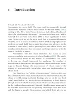
l Goals & Objectives
u What information is needed by
planners and decision-makers?
u What type of models are needed to
provide this information?
l Data Availability
u What is available?
u What is the quality?
u What models will the data support?
l Budget
u What are financial constraints?
Goals
Goals
Data
Data
Budget
Budget
Water Demand Forecast Approaches
Cost & Complexity
Cost & Complexity
Low
Low
High
High
Trend
Trend
Extrapolation
Extrapolation

Per
Per
Capita
Capita
Unit
Unit
Use
Use
Econometric
Econometric
Trend Extrapolation
0
50
100
150
200
250
1
98
0
1
98
5
19
9
0
19
9
5
2000

2005
2
01
0
2
01
5
20
2
0
Historical
Linear Trend
Pros:
l Only historical demand data
required
l Very low cost
Cons:
l Assumes past trend carries
into the future
l No ability to “explain” water
demands
l Cannot account for changes
in demographics, weather, or
other factors
Approach:
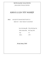
Per Capita
Approach:
l Divide historical total demand by
population to get per capita use
l Multiply per capita use by

projected population to get future
demand
Pros:
l Simple to understand
l Allows for main driver,
population, to be accounted
for
Cons:
l Demands do not always
follow population growth
l Does not account for factors
such as price, income, types
of housing, employment
trends, or other influencers of
demand
0
100,000
200,000
300,000
400,000
500,000
600,000
700,000
800,000
1980 1983 1986 1989 1992 1995 1998 2001 2004
0
500,000
1,000,000
1,500,000
2,000,000

2,500,000
3,000,000
3,500,000
4,000,000
4,500,000
Water Demand
Population
Unit Use
Pros:
l Allows for all major sectors
& drivers of water demand
to be accounted for
Cons:
l Water use factors, such as
weather, income, price and
others are not incorporated
Approach:
l Get sector demands (e.g., single-
family, multifamily, non-
residential)
l Divide each sector demands by
appropriate drivers (e.g., housing
or employment) to get unit use
Example:
Example:
Single
Single
-
-
family demand = 150 MGD

family demand = 150 MGD
Single
Single
-
-
family homes = 500,000
family homes = 500,000
Unit use = 150,000,000 gal/day
Unit use = 150,000,000 gal/day
÷
÷
500,000 homes =
500,000 homes =
300 gallons/home/day
300 gallons/home/day
Econometric
Approach:
l Statistically correlates sector
water demands with factors that
influence those demands
l For each water use factor, an
elasticity is estimated
l Elasticities change the unit use
rates over time
Pros:
l Site specific statistical
estimation of demand and
its influencers
l Significant ability to
“explain” water use over

time
l Allows for probabilistic
results
Cons:
l Data intensive
l More costly to produce than
other methods
Elasticity Defined:
A statistical rate of change that
describes how a water use factor
influences demand. A price
elasticity of -0.10 means that a
ten percent increase in real price
will result in a one percent
decrease in water demand
Example Elasticities
The following are elasticities estimated for water use factors from almost
200 statistical water demand equations in the United States
Water Use Factor
Water Use Factor
Winter Season
Winter Season
Summer Season
Summer Season
Marginal Price
Marginal Price
-
-
0.050
0.050

to
to
-
-
0.250
0.250
-
-
0.150 to
0.150 to
-
-
0.350
0.350
Income
Income
+0.200
+0.200
to +0.500
to +0.500
+0.300 to +0.600
+0.300 to +0.600
Household Size
Household Size
+0.400
+0.400
to +0.600
to +0.600
+0.200 to +0.500
+0.200 to +0.500

Housing Density
Housing Density
-
-
0.200
0.200
to
to
-
-
0.500
0.500
-
-
0.400 to
0.400 to
-
-
0.800
0.800
Precipitation
Precipitation
-
-
0.010
0.010
to
to
-
-

0.150
0.150
-
-
0.050 to
0.050 to
-
-
0.200
0.200
Temperature
Temperature
+0.300
+0.300
to +0.600
to +0.600
+0.800 to +1.500
+0.800 to +1.500
(
(
Paredes
Paredes
, 1996).
, 1996).
Probabilistic Results from Econometric
Forecasts
2010
2060
2030
Water Demand (mgd)

B
a
s
e
l
i
n
e

F
o
r
e
c
a
s
t
B
a
s
e
l
i
n
e

F
o
r
e

c
a
s
t
R
a
n
g
e

d
u
e

t
o

h
i
s
t
o
r
i
c
a
l

w
e

a
th
e
r
R
a
n
g
e

d
u
e

t
o

h
i
s
t
o
r
i
c
a
l

w
e

a
th
e
r
R
a
n
g
e

d
u
e

t
o

d
e
m
o
g
r
a
p
h
i
c
R
a

n
g
e

d
u
e

t
o

d
e
m
o
g
r
a
p
h
i
c
g
r
o
w
t
h

u

n
c
e
r
t
a
i
n
t
y
g
r
o
w
t
h

u
n
c
e
r
t
a
i
n
t
y
R
a

n
g
e

d
u
e

t
o

c
l
i
m
a
t
e

c
h
a
n
g
e
R
a
n
g
e

d
u
e

t
o

c
l
i
m
a
t
e

c
h
a
n
g
e
75%
75%
50%
50%
95%
95%
Ranges of Uncertainty: @Risk Model vs. All High/All Low Assumptions
0

25
50
75
100
125
150
175
200
225
250
1995 2000 2005 2010 2015 2020 2025 2030 2035 2040 2045 2050 2055 2060
Annual Average MGD
90th-95th
85th-90th
80th-85th
75th-80th
70th-75th
65th-70th
60th-65th
55th-60th
50th-55th
45th-50th
40th-45th
35th-40th
30th-35th
25th-30th
20th-25th
15th-20th
10th-15th
5th-10th

Zero-5th
Percentile
Actual
Demand
Firm Yield
Oal Forecas
t
5th Percentile Forecas
t
All Low (≈0% probability)
All High (≈0% probability)
95th Percentile Forecas
t
Draft Official Forecas
t
Growth in Population & Water
Consumption
0
200,000
400,000
600,000
800,000
1,000,000
1,200,000
1,400,000
0
30
60
90
120

150
180
210
1975 1980 1985 1990 1995 2000 2005
Population
Annual MGD
Population
Total Consumption
Billed
Consumption
Non-Rev
Per capita Implications
Actual and Forecast Water Consumption Per Capita: Seattle & Non-CWA
With and Without Programmatic Conservation after 2005
0
20
40
60
80
100
120
140
160
180
1990 1995 2000 2005 2010 2015 2020 2025 2030 2035 2040 2045 2050 2055 2060
GPD per Person
GPD per Person
WITHOUT
Conservation
GPD per Person

WITH
Conservation
Actual GPD
per Person
Impact of All Forms of Conservation
on Past and Forecast Water Demand
0
25
50
75
100
125
150
175
200
225
250
1975 1980 1985 1990 1995 2000 2005 2010 2015 2020 2025 2030
Annual MGD
Unattributed Savings
Transitory Savings
Conservation Programs
Plumbing Code
Rate Impacts
System Operation Improvements
1990 Forecast with No
Conservation
Actual
Demand
2007 Forecast with

Conservation
38
40
42
44
46
48
50
52
54
2004 2005 2006 2007 2008 2009 2010 2011 2012
2004TSP
Composite
Projecti on
2004
Financial
Forecast
Actual
Demand
Cascade average daily demand
(mgd)
Three-stage supply evaluation
Screening:
Eliminates projects that are not feasible
and do not warrant further investigation,
using pass/fail criteria
Multi-Criteria Analysis
:
More refined analysis that evaluates
projects using multiple ranking criteria

Detailed Evaluation
Detailed infrastructure and financial evaluation
of the highest ranked projects
# Name Description
10 Everett -
Sultan River
Supply
Expansion
Increase withdrawals from the Sultan River
Basin (need further information on
conveyance concept)
13 Lake
Sammamish
Develop supply from Lake Sammamish with
Treatment Facility
14 Off-Stream
Storage
Impound water from tributaries in the high
flow season and used to satisfy irrigation
needs
18 OASIS –
Phases 1 & 2
Members utilize Lakehaven's ASR program
water (directly, or via water swap between
green river supply and ASR groundwater)
22 Water from
Puget Sound
Construct a desalination plant either alone or
in partnership with others. Construct
conveyance.

25 South
Treatment
Plant
Expand reclaimed water uses in Tukwila from
South Plant.
30 Rainwater
Collection
Collect and store rainwater fo up to 7 Golf
Courses
33 Regional
Unaccounted-
for Water
Reduce transmission and storage losses from
regional facilities
Legal
Permit.
W. Rights
Tech.
Yield
Location
Overview of Approach
l Identify water supply alternatives
l Determine levelized unit costs to capture life-
cycle costs to utility, both capital and O&M
l Determine non-monetary values, benefits and
impacts of each alternative using value model
l Compare alternatives using value scores and
levelized unit costs
Value Modeling Overview
l Identify objectives or criteria important in selecting

preferred alternative
l Define how these objectives will be measured and
scored—can be simple 1-5 scale with endpoints
defined.
l Assign weights to the objectives
l Score each alternative, or package of alternatives, and
document reasoning
l Determine single value score
l Test sensitivity of results to weights and scores
l Criterium Decision Plus (CDP) software aids in this
process
Political
Acceptability
Public
Acceptability
(Stakeholders)
Public
Trust
30
Built
Environment
Natural
Environment
Environmental
Acceptability
of Construction
20
Timing
Reliability
Leads to Other Sources

Asset
Reliability
20
Legal/
Regulatory
30
Ease of Source
Development
45
Natural
Environment
Secondary
Impacts and
Benefits/
Sustainability
Environmental
Acceptability
25
System
Robustness
Operational
Flexibility
Security
Asset
Reliability
25
Public
Trust
25
Regulatory

Compliance
Source
Compatibility
Public Health/WQ
15
Social
(Lifestyles)
10
System
Operation
55
Value Model
SPU Water Supply
System Options
Value Model
Criteria and Weights
Value Model
Contributions to Value Score
0.0
0.2
0.4
0.6
0.8
0.0
0.2
0.4
0.6
0.8
Legal/Regulatory
Env. Acceptability

Public Trust (Develop)
Asset Reliability (Ops)
Pub. Health (WQ)
Asset Reliability (Dev)
Others
1.0 is best outcome, with positive consequences
0.0 is worst outcome, with negative impacts
Cedar Dead
Storage
Lake Youngs
Snoqualmie
Aquifer
SFTolt 1695
SF Tolt 1660
NF Tolt Diversion
Conservation
0.0
0.1
0.2
0.3
0.4
0.5
0.6
0.7
0.8
0.9
1.0
0.0 0.5 1.0 1.5 2.0 2.5 3.0 3.5 4.0
Levelized Unit Cost (PVm$/PVmgd)
a

Value Score
a
Calculated assuming all sources online in 2050. 4 mgd conservation program begins in 2045 and phases
in over a 10-year period.
Low Value
Low Cost
High Value
Low Cost
Low Value
High Cost
High Value
High Cos
t
SPU Water Supply Sources
Value-Cost Tradeoff
SPU Water Supply Sources
Value-Cost Tradeoff

Cedar Dead
Storage
Lake Youngs
Drawdown
Snoqualmie
Aquifer
SF Tolt 1695
SF Tolt 1660
North Fork Tolt
Conservation*
0.0
0.1

0.2
0.3
0.4
0.5
0.6
0.7
0.8
0.9
1.0
0.0 0.5 1.0 1.5 2.0 2.5 3.0 3.5 4.0
Levelized Unit Cost (PVm$/PVmgd)
a
Value Score
a
Calculated assuming all sources online in 2050.
*4 mgd conservation program begins in 2045 and phases in over a 10-year period.
Low Value
Low Cost
High Value
Low Cost
Low Value
High Cost
High Value
High Cost
Value: 0.478 - 0.500
Cost: $5.80 - $10.94
Reclaimed Water Projects
Preliminary Ranking of Supply Options
20%
20%

20%
13%
12%
10%
5%
0.00 0.10 0.20 0.30 0.40 0.50 0.60 0.70 0.80 0.90
Replacement Wells, No Treatment
Treatment for Inactive, Sustainable Wells
Within City Wells, No Treatment
Within City Wells, Treatment
Within City Wells, Treatment, Not Sustainable
Large Seawater Desalination
Small Seawater Desalination
Outside City Wells, No Treatment (Indian Spr)
Outside City Wells, No Treatment (N. of River)
Surface Water Direct Use with Treatment
Surface Water with ASR Wells
Cost
Supply
Legal
Institutional
Environment
Regulatory
Permitting
Climate Change Planning
l Downscaling of International Climate Models
l Up scaling of Local Hydrologic Models
l Used the Expertise of the University of
Washington Climate Impacts Group
l Used Scenario Planning Because of the

Uncertainties