schaum s easy outline of principles of economics based on schaum s outline of theory and problems of principl phần 4 potx
Bạn đang xem bản rút gọn của tài liệu. Xem và tải ngay bản đầy đủ của tài liệu tại đây (253.61 KB, 15 trang )
of $50 billion equals 0.80. For consumption function CЈ, the MPC = 0.80
for each change in disposable income. It is constant for any linear con-
sumption function since the MPC is the consumption function’s slope,
and all straight lines have a constant slope.
Note!
Consumers comprise the largest percentage of ag-
gregate spending, so their actions are very impor-
tant to the strength of the economy.
Investment
Gross investment is the least stable component of aggregate spending and
a principal cause of the business cycle. In calculating GDP, investment
consists of residential construction; nonresidential construction (offices,
hotels, and other commercial real estate); producers’ durable equipment;
and changes in inventories. While the rate of interest is only one of many
variables that influence investment decisions, it is customary to present
investment demand as a negative function of the interest rate, holding
constant the other variables which influence the decision to invest. Thus,
a lower interest rate is associated with a higher level of investment, and
vice versa.
Holding other variables constant, we expect that at a lower rate of in-
terest (1) more households are financially able to carry a mortgage, and
a greater number of housing units will be demanded; (2) businesses are
more willing and able to purchase durable equipment and to carry larger
inventories; and (3) real estate developers find that there are a larger num-
ber of purchasers for newly constructed commercial real estate.
Net Exports
Gross exports are the value of goods and services produced in a home
country and sold abroad, i.e., they are the value of foreign spending on
U.S produced goods and services. Gross imports are the value of U.S.
40 PRINCIPLES OF ECONOMICS
purchases of goods and services produced in other countries. When com-
modities are imported, some of the consumption and gross investment
spending is for foreign-produced rather than U.S produced goods. Im-
ports thereby lower aggregate spending on domestically produced goods.
Net exports are the value of gross exports less gross imports, i.e., the
net addition to domestic aggregate spending that results from importing
and exporting goods and services. Net exports are positive when the
home country exports more than it imports, and negative when the home
country imports more than it exports.
Numerous variables affect a country’s imports and exports. A coun-
try’s imports are related to its level of income, foreign exchange rate, do-
mestic prices relative to prices in foreign countries, import tariffs, and
restrictions on imported goods. Exports are influenced by the same vari-
ables, except that the income levels of foreign countries rather than that
of the home country affect the amount exported. Because these variables
change with time, it is reasonable to expect a country’s net export balance
to change over time.
You Need to Know
In the United States net exports are often referred
to as the trade deficit because U.S. imports have
been greater than exports for some time.
Government Taxes and Expenditures
Government spending increases when Congress passes legislation au-
thorizing new spending. Tax revenues finance this government spending
and government transfer payments to the private sector. Government
transfer payments (in the form of unemployment insurance, social secu-
rity payments, and various government assistance programs) can be
viewed as a negative tax. Net tax revenues consist of income taxes plus
lump-sum taxes less transfer payments. Net tax revenues fall when trans-
fer payments increase, and rise when greater per capita taxes are imposed.
CHAPTER 4: Consumption, Investment, Exports and Government 41
With respect to income tax receipts, net tax revenues increase when out-
put increases and more taxes are collected or when government imposes
a higher income tax rate.
Don’t Forget!
Income tax receipts may decrease if the economy
slows, not just because Congress cuts tax rates.
True or False Questions
1. A change in disposable income causes an equal change in con-
sumption.
2. Investment spending is the most unstable component of aggregate
spending.
3. Consumption and investment spending in the national income ac-
counts is solely for domestically produced goods and services.
4. Imports by a country are unrelated to its level of GDP.
Answers: 1. False; 2. True; 3. False; 4. False
Solved Problems
Solved Problem 4.1 Suppose the economy’s consumption function is
specified by the equation C = $50 + 0.80Y
d
.
a. Find consumption when disposable income (Y
d
) is $400, $500, and
$600.
b. Plot this consumption equation and label it CЈ.
c. Use the plotted consumption function to find saving when dispos-
able income is $400, $500, and $600.
d. What amount of consumption for consumption function CЈ is au-
tonomous, and what amount is induced when disposable income is $400?
$500? $600?
Solution:
a. Consumption for each level of disposable income is found by sub-
stituting the specified disposable income level into the consumption
42 PRINCIPLES OF ECONOMICS
equation. Thus, for Y
d
= $400, C = $50 + 0.80($400) = $50 + $320 = $370.
So, C is $450 when Y
d
= $500, and $530 when Y
d
= $600.
b. The linear consumption function C = $50 + 0.80Y
d
is plotted in
Figure 4-2.
c. Saving is the difference between disposable income and con-
sumption. Using the calculation from part a., we find that saving is $30
when Y
d
is $400 (Y
d
− C = S = $400 − $370 = $30), $50 when Y
d
is $500,
and $70 when Y
d
is $600. Saving is the difference between the con-
sumption line and the 45Њ line at each level of disposable income in Fig-
ure 4-2. Thus, reading up from the $400 income level, we find that C is
$370; the distance from consumption function CЈ to the 45Њ line at the
$400 income level is $30—the amount of saving.
d. Autonomous consumption is the amount consumed when dispos-
able income is 0. In Figure 4-2, autonomous consumption is $50, the
amount consumed when the consumption line CЈ intersects the vertical
axis and disposable income is 0. Since autonomous consumption is un-
related to income, autonomous consumption is $50 for all levels of in-
come. Induced consumption is the amount of consumption that depends
upon the receipt of income. Consumption is $370 when disposable in-
CHAPTER 4: Consumption, Investment, Exports and Government
43
Figure 4-2
come is $400. Since $50 is consumed regardless of the income level, $320
of the $370 level of consumption is induced by disposable income. In-
duced consumption is $400 when disposable income is $500, and $480
when disposable income is $600.
Solved Problem 4.2 What will happen to consumption function CЈ in
Figure 4-2 when:
a. Consumers consider their job secure and therefore become more
confident about the future level of disposable income?
b. Credit card issuers implement tighter credit standards and con-
sumers are less able to buy goods and services on credit?
c. Consumers expect the price level to increase 10 percent by year
end?
Solution:
a. Consumers become more willing to consume their current dispos-
able income. Consumption function CЈ in Figure 4-2 shifts upward to CЉ,
and consumption is greater for each level of disposable income.
b. Some consumers are no longer able to borrow to purchase goods
and services in the current period. The consumption function will shift
downward from CЉ to CЈ. Consumption is lower for each level of dis-
posable income.
c. Consumers reschedule future purchases to the current period be-
cause of the expected rise in prices for goods and services. Consumption
function CЈ shifts upward to CЉ.
Solved Problem 4.3 Variables other than the rate of interest affect gross
investment. Changes in these other variables cause investment demand
to shift downward or upward. What should happen to the economy’s in-
vestment demand when there is a change in the following variables?
a. There is an increase in consumer confidence.
b. Manufacturers’ utilization of existing capacity declines.
c. There is an increase in vacancy rates in commercial buildings.
Solution:
a. Investment demand should shift upward. Housing sales should in-
crease as consumers become more confident; builders would construct
more new housing to meet this increased demand.
b. Investment demand should shift downward. Businesses’ purchas-
es of durable equipment should fall since such purchases would expand
44 PRINCIPLES OF ECONOMICS
productive capacity and there is no need to expand productive capacity
when utilization of existing capacity is declining.
c. Investment demand should shift downward. Increased vacancy
rates for existing commercial buildings indicate that there will be diffi-
culty selling newly constructed commercial real estate. Thus, commer-
cial real estate construction will decline.
Solved Problem 4.4 What is the difference between a lump-sum tax and
an income tax?
Solution: A lump-sum tax is a fixed-sum tax that is unrelated to income.
An income tax is related directly to earned income. In the case of a pro-
portional income tax the government collects a fixed percent of income
earned, while for a progressive income tax the rate of taxation increases
with the level of income. Lump-sum taxes and proportional and progres-
sive income taxes are illustrated in Figure 4-3. Note that lump-sum tax-
es remain at $1,000 as income increases from $10,000 to $11,000. When
there is a 10 percent proportional income tax rate, tax payments increase
from $1,000 to $1,100 as income increases from $10,000 to $11,000.
When the tax rate is 10 percent on the first $10,000 earned and 20 per-
cent on income greater than $10,000, tax payments increase from $1,000
to $1,200 when income increases from $10,000 to $11,000.
CHAPTER 4: Consumption, Investment, Exports and Government
45
Figure 4-3
Chapter 5
Traditional
Keynesian
Approach to
Equilibrium
Output
In This Chapter:
✔ Keynesian Model of Equilibrium
Output
✔ Income-Expenditure Model of
Equilibrium Output
✔ Leakage-Injection Model of
Equilibrium Output
✔ The Multiplier
✔ Changes in Equilibrium Output
When Aggregate Supply Is
Positively Sloped
46
Copyright 2003 by The McGraw-Hill Companies, Inc. Click Here for Terms of Use.
✔ True or False Questions
✔ Solved Problems
Keynesian Model of Equilibrium Output
John Maynard Keynes developed the framework for modern-day macro-
economics in the 1930s. Because there was considerable unemployment
at that time, he assumed that changes in aggregate demand have no effect
upon the price level as long as output is below the full-employment lev-
el, i.e., as long as aggregate supply is horizontal. A positive GDP gap—
where real GDP is below potential GDP—is identified as a recessionary
gap and is the distance between equilibrium output and full-employment
output on an AD-AS graph. An inflationary gap exists when there is ex-
cessive aggregate spending, such that aggregate demand intersects the
Keynesian aggregate supply curve in the positively sloped region beyond
full-employment output. This results in an increase in the price level.
Income-Expenditure Model of Equilibrium
Output
The Keynesian model of output can be expressed
as a circular flow of income and output between
businesses and individuals. In a capitalist, free-
market economy, individuals own, directly or indi-
rectly, the economy’s economic resources (land, la-
bor, and capital). Businesses hire resources to produce output and pay
individuals a money income for the services of these resources in the form
of wages, rent, interest, and profits. Individuals in turn spend their mon-
ey income and purchase output. Assuming no supply constraints (when
aggregate supply is horizontal), we can expect businesses to supply out-
put as long as the receipts from selling output equal the payments made
by businesses to the owners of economic resources and the owners of the
business firms.
CHAPTER 5: Keynesian Approach to Equilibrium Output 47
Note!
The circular flow of income and output helps to ex-
plain why we should all study economics because
one person’s actions have repercussions for oth-
ers.
The circular flow of income and expenditure can be used to find the
economy’s equilibrium level of output. The market value of final output
for a hypothetical economy appears in column 1 of Table 5.1.
Assuming a capitalist system with no government spending or tax-
es, the value of output in column 1 is also the disposable income of indi-
viduals since individuals receive all the payments made to the factors of
production. Aggregate spending in column 5 is the sum of consumer
spending (column 2), investment spending (column 3), and net exports
(column 4). Note that consumer spending increases with the level of out-
put and thus the level of personal disposable income, as discussed in
Chapter 4. Investment and net exports are assumed here to be unrelated
to the output level and remain constant. The equilibrium level of output
is $800 billion since this is the only level of production at which output
equals aggregate spending. This equilibrium condition is depicted in col-
48 PRINCIPLES OF ECONOMICS
Table 5.1
(in Billions of $)
umn 6 by the absence of production shortages or surpluses. At output lev-
els below $800 billion there is a shortage of output (aggregate spending
is greater than production), while at output levels greater than $800 bil-
lion there is surplus production.
The income-expenditure approach to output can be presented graph-
ically beginning with the linear consumption function and the 45Њ line en-
countered in Chapter 4. Adding investment spending and net exports
shifts the linear consumption function upward to the aggregate spending
line (C + I + X
n
). Aggregate spending equals output at only one level of
output, determined by the intersection of the 45Њ line and the aggregate
spending line. It can be shown that increases (upward shifts) or decreases
(downward shifts) of aggregate spending increase or decrease the econ-
omy’s equilibrium level of output.
Example 5.1
The equilibrium level of output can be found algebraically by equating
output and aggregate spending. Suppose the equation for the linear con-
sumption function is C = $70 + 0.8Y; I is $120 and X
n
= 0. Equilibrium
output is found by solving Y = C + I + X
n
for Y.
Y = C + I + X
n
Y = $70 + 0.8Y + $120 + 0
Y − 0.8Y = $70 + $120 + 0
0.2Y = $190
Y = $190.2 = $950
Leakage-Injection Model of Equilibrium Output
The leakage-injection model of equilibrium output fo-
cuses on saving and gross imports as leakages from the
circular flow and on investment and gross exports as
spending injections. Leakages depress aggregate spend-
ing, while injections increase aggregate spending. For
example, spending on domestic output declines when in-
dividuals buy more imported rather than domestically produced com-
modities. An equilibrium level of output exists in the leakage-injection
model when the sum of leakages equals the sum of injections.
CHAPTER 5: Keynesian Approach to Equilibrium Output
49
The paradox of thrift demonstrates that increases or decreases in con-
sumers’ desire to save, ceteris paribus, affect the economy’s output lev-
el but not its saving level. Suppose that there are no exports or imports
and that the government neither taxes nor spends. Individuals begin to
save more of their income, which is a leakage. If investment does not in-
crease, leakages will not equal injections. However, output will be de-
creased because individuals are not spending as much with more saving.
Since output becomes income to individuals, income will decrease until
saving equals investment again, i.e., leakages equal injections. If invest-
ment does not change, saving must end up at its initial value. Individuals
may be saving a greater percentage of their income, but they have less in-
come. So saving stays the same while output decreases. Saving has hurt
the economy, thus the paradox.
Remember
The paradox of thrift explains why it
is good for an individual to save, but
not necessarily good for the econo-
my in general.
The Multiplier
Shifts of the aggregate spending curve result in a change in the equilibri-
um level of output that is several times larger than the initial shift of the
curve. This multiplied effect upon output arises from consumption’s pos-
itive relationship to income. For example, an increase in investment
spending of $10 billion will raise consumers’ income by $10 billion,
which results in numerous rounds of induced consumer spending. The
new recipients of the $10 billion will consume 80 percent or $8 billion (if
the MPC = 0.80). This new $8 billion in spending will become new in-
come to individuals who will also spend 80 percent or $6.40 billion, and
so on.
50 PRINCIPLES OF ECONOMICS
Important!
The multiplier is extremely important in explaining
how strong an impact one person’s actions can
have upon the economy.
The value of the multiplier (k) is found by relating the change in out-
put (∆Y) to the initial change in aggregate spending. The value of the mul-
tiplier can also be found from the equation k = 1/(1 − MPC). Thus, the
multiplier is 5 if the MPC = 0.80.
Changes in Equilibrium Output When
Aggregate Supply Is Positively Sloped
When the aggregate supply curve is positively sloped, increases in ag-
gregate demand raise both equilibrium output and the price level, even
though output may be below its full-employment level. The $50 billion
outward shift of aggregate demand from ADЈ to ADЉ in Figure 5-1 rais-
es equilibrium output $40 billion rather than $50 billion because of a pos-
itively sloped aggregate supply curve.
If the aggregate supply curve had been horizontal in this range and
the price level had remained at p
1
, equilibrium output would have in-
creased $50 billion, an amount equal to the shift in the aggregate demand
curve. It therefore follows that an increase in aggregate spending, when
aggregate supply is positively sloped, has a smaller multiplier effect since
the increase in the price level decreases wealth (which limits the expan-
sion of induced consumer spending), causes higher interest rates (which
slow investment spending), and reduces the purchasing power of the
home currency (which increases imports and decreases exports).
True or False Questions
1. An inflationary gap exists when output is above the economy’s
equilibrium level of output.
CHAPTER 5: Keynesian Approach to Equilibrium Output
51
2. A production shortage exists when the output level is to the right
of the point of intersection of the aggregate spending line and the 45Њ line.
3. A decrease in saving, ceteris paribus, results in a decrease in the
equilibrium level of output.
4. A $5 billion increase in investment spending results in a $50 bil-
lion increase in the equilibrium level of output when the MPC is 0.90 and
aggregate supply is horizontal.
5. An equilibrium level of output exists when output is $550 billion,
investment spending is $70 billion, net exports equal $30 billion, and the
consumption function is C = $10 billion + 0.80Y.
Answers: 1. False; 2. False; 3. False; 4. True; 5. True
Solved Problems
Solved Problem 5.1 Suppose individuals own all businesses and eco-
nomic resources, government does not tax or spend, and the business sec-
tor produces 500 units at an average price of $1.50 per unit.
a. What is the money value of output?
52 PRINCIPLES OF ECONOMICS
Figure 5-1
b. What is the money income of individuals?
c. Find consumer spending when individuals spend 90 percent of
their income.
d. What money revenues are received by the business sector from
consumer spending?
e. What is the relationship of the cost of producing output and the
money receipts of businesses when there are only consumer expendi-
tures? What should happen to the level of output?
Solution:
a. The money value of output equals the output times the average
price per unit. The money value of output is $750 (500 × $1.50).
b. Since individuals receive an amount equal to the money value of
output, their money income is $750.
c. Individuals are spending $675—0.90 times their $750 money in-
come. There is a $75 saving leakage from the circular flow.
d. Business revenues equal the sum of aggregate spending. Since in-
dividuals are the only source of spending, revenues equal $675.
e. Businesses are making payments of $750 to produce output, while
individuals are purchasing only $675 of what is produced. Because busi-
ness firms are left holding unsold output valued at $75, they can be ex-
pected to decrease output.
Solved Problem 5.2 Suppose there are no gross imports, gross exports,
government taxes, or government expenditures for Figure 5-2.
a. What is the equilibrium level of output?
b. What is the level of saving and investment when output is $400,
$500, and $600?
c. There being no gross imports or exports, what is the relationship
of saving leakages and investment injections when output is above and
below the equilibrium output?
Solution:
a. The equilibrium level of output is $500, determined by the point
of intersection of the aggregate spending line (C + I)Ј and the 45Њ line.
b. Saving at each level of output is the difference between the income
received and the amount consumed; in the graph, it is the difference be-
tween the consumption line CЈ and the 45Њ line. Consumption is $350 and
saving is $50 when Y = $400. Saving is $100 when Y = $500, and $150
CHAPTER 5: Keynesian Approach to Equilibrium Output
53
when Y = $600. Investment spending is $100, the distance between the
consumption line and the aggregate spending line.
c. When output is below the equilibrium level of output, investment
injections are greater than saving leakages, e.g., saving is $50 when Y =
$400 while I = $100. When output is above the equilibrium level of out-
put, investment injections are smaller than saving leakages, e.g., saving
is $150 when Y = $600 while I = $100. At equilibrium, saving leakages
equal investment injections.
Solved Problem 5.3
a. Find the value of the multiplier when MPC = 0.50, 0.75, and 0.80.
b. Find the relationship between the multiplier and the MPC.
c. Find the change in the equilibrium level of output when there is a
$10 increase in net export spending and the MPC = 0.50, 0.75, and 0.80.
54 PRINCIPLES OF ECONOMICS
Figure 5-2