the behavior of stock market prices eugene f fama the journal phần 5 pdf

85
BEHAVIOR OF STOCK-MARKET PRICES
that the academic researcher is not in-
terested in whether the dependence in
series of price changes can be used to in-
crease expected profits. Rather, he is
primarily concerned with determining
whether the independence assumption is
an
exact
description of reality. In essence
he proposes that we treat independence
as a extreme null hypothesis and test it
accordingly.
At this time we will ignore important
counterarguments as to whether a strict
test of an extreme null hypothesis is like-
ly to be meaningful, given that for prac-
tical purposes the hypothesis would seem
to be a valid approximation to reality for
both
the statistician and the investor.
We simply note that a signs test applied
to the profit figures in column (1) of
Table
16
would not reject the extreme
null hypothesis of independence for any
of the standard significance levels. Six-
teen of the profit figures in column (1)
are positive and fourteen are negative,

which is not very far from the even split
that would be expected under a pure ran-
dom model without trends in the price
levels.
If
we allowed for the long-term
upward bias of the market, the results
would conform even more closely to the
predictions of the strict null hypothesis.
Thus the results produced by the
filter
technique do not seem to overturn the
independence assumption of the random-
walk model, regardless of how strictly
that assumption is interpreted.
Finally, we emphasize again that these
results must be regarded as preliminary.
Many more complicated analyses of the
filter technique are yet to be completed.
For example, although average profits
per filter do not compare favorably with
buy-and-hold, there may be particular
filters which are consistently better than
buy-and-hold for all securities. We pre-
fer, however, to leave such issues to
a
later paper. For now suffice it to say that
preliminary results seem to indicate that
the filter technique does not overturn the
independence assumption of the random-

walk model.
D. DISTRIBUTION OF SUCCESSORS
TO LARGE VALUES
Mandelbrot
137,
pp. 418-191 has sug-
gested that one plausible form of de-
pendence that could partially account
for the long tails of empirical distribu-
tions of price changes is the following:
Large changes may tend to be followed
by large changes, but of random sign,
whereas small changes tend to be fol-
lowed by small
changes.36 The economic
rationale for this type of dependence
hinges on the nature of the information
process in
a
world of uncertainty. The
hypothesis implicitly assumes that when
important new information comes into
the market, it cannot always be evalu-
ated precisely. Sometimes the immediate
price change caused by the new informa-
tion will be too large, which will set in
motion forces to produce a reaction. In
other cases the immediate price change
will not fully discount the information,
and impetus will be created to move the

price again in the same direction.
The statistical implication of this hy-
pothesis is that the conditional probabil-
ity that tomorrow's price change will be
large, given that today's change has been
large, is higher than the unconditional
probability of a large change. To test
this, empirical distributions of the imme-
diate successors to large price changes
have been computed for the daily
differ-
Although the existence of this type of price be-
havior could not be used by the investor to increase
his expected profits, the behavior does fit into the
statistical definition of dependence. That is, knowl-
edge of today's price change does condition our pre-
diction of the
size,
if not the
sign,
of tomorrow's
change.
86
THE JOURNAL OF BUSINESS
ences of ten stocks. Six of the stocks were
quency distributions of all price changes.
chosen at random. They include Allied
It shows for each stock the number and
Chemical, American Can,
Eastman Ko-

relative frequency of observations in the
dak, Johns Manville, Standard Oil of
distribution of successors within given
New Jersey, and U.S. Steel. The other
ranges of the distribution of all price
four were chosen because they showed
changes. For example, the number in
longer than average tails in the tests of
column (1) opposite Allied Chemical in-
Sections
I11
and IV. A large daily price
dicates that there are twenty-seven ob-
change was defined as a change in log
servations in the distribution of succes-
price greater than
0.03
in absolute value.
sors to large values that fall within the
The results of the computations are
intersextile range of the distribution of
shown in Table
17.
The table is arranged
all price changes for Allied Chemical.
to facilitate a direct comparison between
The number in column (6) opposite Al-
the frequency distributions of successors
lied Chemical indicates that
twenty-

to large daily price changes and the fre-
seven observations are 55.1 per cent of
TABLE
17
Intersextile
1
2 Per Cent
1
1
Per Cent
1
>
1 Per Cent
1
Total
Stock
(1) (21
(31
4
(5)
Number
Allied Chemical

27
46
48
1
49
American Can

13
26
27 5
32
A.T.&T

4
12
14
2
16
Eastman Kodak.

25
35
39
5
44
Goodyear

40
66
66
4
70
Johns Manville.

38
62
63 3

66
Sears

14
25
28
3
3 1
Standard Oil (N. J.)
.
.
11
18
18
2
20
United Aircraft.

49 78
84
4
88
U.S. Steel

14
2
7
3 1 5
36
Frequency

(6)

(7)
(8)
(9)

Expected frequency.
Allied Chemical

0.6667
.5510
0.9600
.9388
0.9800
.9796
0.0200
.0204
American Can.

.4063
.8125 .8438
.I562
A.T.&T.

.2500 .7500 .8750
.I250
Eastman Kodak.

.5682 .7955
.8864 .I136

Goodyear.

Johns Manville.

.5714
.5758
.9429
.9394
.9429
.9545
.0571
.0455
Sears.

.4516
.8065 .9032
.0968
Standard Oil (N.
J.).
.
United Aircraft

.5500
.5568
.9000
,8864
.9000
.9545
.I000
.0455

U.S. Steel

0.3889 0.7500
0.8611 0.1389
*
Number and freouencv of observations in the distributions of successors within given ranges
of the distributions oi'all chanacs. The ranges arc defined
as
folloks: Intersestilt
='o
8; frdii
-0.1; fractilc:
2
pcr ccnt
=
0.98fractilt
0.02
fractile; 1 per cent
=
0.99fract1lt -4.01 fracjilc.
The fractiles arc the fractilcs of the distributions of all price changes and not of the distrlbut~ons
of successors to large changes.
87
BEHAVIOR OF STOCK-MARKET PRICES
the total number of successors to large
values, whereas the distribution of all
price changes contains, by definition,
66.7 per cent of its observations within
its intersextile range. Similarly, the num-
ber in column

(9)
opposite Goodyear
indicates that in the distribution of suc-
cessors
5.7
per cent of the observations
fall outside of the 1 per cent range,
whereas by definition only
2
per cent of
the observations in the distribution of
all changes are outside this range.
It
is evident from Table 17 that the
distributions of successors are flatter and
have longer tails than the distributions
of all price changes. This is best illus-
trated by the relative frequencies. In
every case the distribution of successors
has less relative frequency within each
fractile range than the distribution of all
changes, which implies that the distribu-
tion of successors has too much relative
frequency outside these ranges.
These results can be presented graphi-
cally by means of simple scatter dia-
grams. This is done for American Tele-
phone and Telegraph and
Goodyear in
Figure

8.
The abscissas of the graphs
show XI, the value of the large price
change. The ordinates show Xz, the price
change on the day immediately following
a large change. Though it is
diEcult
to make strong statements from such
graphs, as would be expected in light of
Table 17, it does seem that the successors
do not concentrate around the abscissas
of the graphs as much as would be ex-
pected if their distributions were the
same as the distributions of all changes.
Even a casual glance at the graphs shows,
however, that the signs of the successors
do indeed seem to be random. Moreover,
these statements hold for the graphs of
the securities not included in Figure
8.
In sum, there is evidence that large
changes tend to be followed by large
changes, but of random sign. However,
though there does seem to be more
bunching of large values than would be
predicted by a purely independent mod-
el, the tendency is not very strong. In
Table 17 most of the successors to large
observations do fall within the intersex-
tile range even though more of the suc-

cessors fall into the extreme tails than
would be expected in a purely random
model.
E.
SUMMARY
None of the tests in this section give
evidence of any important dependence in
the first differences of the logs of stock
prices. There is some evidence that large
changes tend to be followed by large
changes of either sign, but the depend-
ence from this source does not seem to
be too important. There is no evidence
at all, however, that there is any depend-
ence in the stock-price series that would
be regarded as important for investment
purposes. That is, the past history of the
series cannot be used to increase the
investor's expected profits.
It
must be emphasized, however, that,
while the observed departures from inde-
pendence are extremely slight, this does
not mean that they are unimportant for
every conceivable purpose. For example,
the fact that large changes tend to be
followed by large changes may not be in-
formation which yields profits to chart
readers; but it may be very important to
the economist seeking to understand the

process of price determination in the
capital market. The importance of any
observed dependence will always depend
on the question to be answered.
VI. CONCLUSION
The purpose of this paper has been to
test empirically the random-walk model
of stock price behavior. The model makes
American Tel.
&
Tel.
Goodyear
89
BEHAVIOR OF STOC K-MARKET PRICES
two basic assumptions:
(1)
successive
price changes are independent, and
(2)
the price changes conform to some prob-
ability distribution. We begin this sec-
tion by summarizing the evidence con-
cerning these assumptions. Then the im-
plications of the results will be discussed
from various points of view.
A. DISTRIBUTION
OF
PRICE CHANGES
In previous research on the distribu-
tion of price changes the emphasis has

been on the general shape of the distri-
bution, and the conclusion has been that
the distribution is approximately Gauss-
ian or normal. Recent findings of
Benoit
Mandelbrot, however, have raised serious
doubts concerning the validity of the
Gaussian hypothesis. In particular, the
Mandelbrot hypothesis states that em-
pirical distributions of price changes con-
form better to stable
Paretian distribu-
tions with characteristic exponents less
than
2
than to the normal distribution
(which is also stable Paretian but with
characteristic exponent exactly equal to
2).
The conclusion of this paper is that
Mandelbrot's hypothesis does seem to be
supported by the data. This conclusion
was reached only after extensive testing
had been carried out. The results of this
testing will now be summarized.
If
the Mandelbrot hypothesis is cor-
rect, the empirical distributions of price
changes should have longer tails than
does the normal distribution. That is, the

empirical distributions should contain
more relative frequency in their extreme
tails than would be expected under a
simple Gaussian hypothesis. In Section
I11
frequency distributions were comput-
ed for the daily changes in log price of
each of the thirty stocks in the sample.
The results were quite striking. The em-
pirical distribution for
each
stock con-
tained more relative frequency in its cen-
tral bell than would be expected under a
normality hypothesis. More important,
however, in
every
case the extreme tails
of the distributions contained more rela-
tive frequency than would be expected
under the Gaussian hypothesis. As a
further test of departures from normal-
ity, a normal probability graph for the
price changes of each stock was also ex-
hibited in Section
111. As would be ex-
pected with long-tailed frequency distri-
butions, the graphs generally assumed
the shape of an elongated
S.

In an effort to explain the departures
from normality in the empirical fre-
quency distributions, two simple compli-
cations of the Gaussian model were dis-
cussed and tested in Section 111. One in-
volved a variant of the mixture of distri-
butions approach and suggested that
perhaps weekend and holiday changes
come from a normal distribution, but
with a higher variance than the distribu-
tion of daily changes within the week.
The empirical evidence, however, did not
support this hypothesis. The second ap-
proach, a variant of the non-stationarity
hypothesis, suggested that perhaps the
leptokurtosis in the empirical frequency
distributions is due to changes in the
mean of the daily differences across time.
The empirical tests demonstrated, how-
ever, that the extreme values in the
frequency distributions are so large that
reasonable shifts in the mean cannot
adequately explain them.
Section IV was concerned with testing
the property of stability and developing
estimates of the characteristic exponent
a
of the underlying stable Paretian proc-
ess.
It

was emphasized that rigorously
established procedures for estimating the
parameters of stable Paretian distribu-
tions are practically unknown because
for most values of the characteristic ex-
ponent there are no known, explicit
90
THE
JOURNAL OF BUSINESS
expressions for the density functions. As
a result there is virtually no sampling
theory available.
It
was concluded that
at present the only way to get satisfac-
tory estimates of the characteristic ex-
ponent is to use more than one estimat-
ing procedure. Thus three different
techniques for estimating
a
were dis-
cussed, illustrated, and compared. The
techniques involved double-log-normal-
probability graphing, sequential compu-
tation of variance, and range analysis. In
a very few cases
a
seemed to be so close
to
2

that it was indistinguishable from 2
in the estimates. In the vast majority of
cases, however, the estimated values were
less than 2, with some dispersion about
an average value close to
1.90.
On the
basis of these estimates of
a
and the re-
sults produced by the frequency distribu-
tions and normal probability graphs,
it
was concluded that the Mandelbrot hy-
pothesis fits the data better than the
Gaussian hypothesis.
33.
INDEPENDENCE
Section
V
of this paper was concerned,
with testing the validity of the independ-
ence assumption of the random-walk
model on successive price changes for
differencing intervals of one, four, nine,
and sixteen days. The main techniques
used were a serial correlation model, runs
analysis, and
-4lexander's filter tech-
nique. For all tests and for all differenc-

ing intervals the amount of dependence
in the data seemed to be either extremely
slight or else non-existent. Finally, there
was some evidence of bunching of large
values in the daily differences, but the
degree of bunching seemed to be only
slightly greater than would be expected
in a purely random model. On the basis
of all these tests it was concluded that
the independence assumption of the ran-
dom-walk model seems to be an adequate
description of reality.
C.
IMPLICATIONS OF INDEPENDENCE
We saw in Section
I1
that a situation
where successive price changes are inde-
pendent is
consistent with
the existence of
an "efficient" market for securities, that
is, a market where, given the available
information, actual prices at every point
in time represent very good estimates of
intrinsic values. We also saw that two
factors that could possibly contribute to-
ward establishing independence are
(1)
the existence of many sophisticated chart

readers actively competing with each
other to take advantage of any depend-
encies in series of price changes, and
(2)
the existence of sophisticated analysts,
where sophistication implies an ability
both to
predict
better the occurrence of
economic and political events which have
a bearing on prices and to evaluate the
eventual effects of such events on prices.
If
his activities succeed in hdping to
establish independence of successive price
changes, then the sophisticated chart
reader has defeated his own purposes.
When successive price changes are inde-
pendent, there can be no chart-reading
technique which makes the expected
profits of the investor greater than they
would be under a naive buy-and-hold
model. Such dogmatic statements do not
apply to superior intrinsic value analysis,
however. People who can consistently
predict the occurrence of important
events and evaluate their effects on
prices will usually make larger profits
than people who do not have this talent.
The fact that the activities of these su-

perior analysts help to make successive
price changes independent does
not
imply
that their expected profits cannot be
greater than those of the investor who
follows a buy-and-hold policy.
Of course, in practice, identifying peo-
ple who qualify as superior analysts is
not an easy task. The simple criterion
91
BEHAVIOR OF STOCK-MARKET PRICES
put forth in Section
I1
was the following:
A
superior analyst is one whose gains
over many periods of time are
consistently
greater than those of the market. There
are many institutions and individuals
that claim to meet this criterion. In a
separate paper their claims will be sys-
tematically tested. We present here some
of the preliminary results for open-end
mutual
funds.37
In their appeals to the public, mutual
funds usually make two basic claims:
(1)

because it pools the resources of many
individuals, a fund can diversify much
more effectively than the average small
investor; and
(2)
because of its manage-
ment's closeness to the market, the fund
is better able to detect "good buys" in
individual securities. In most cases the
first claim is probably true. The second,
however, implies that mutual funds pro-
vide returns higher than those earned by
the market as a whole.
It
is this second
claim that we now wish to test.
The return earned by the "market"
during any time period can be measured
in various ways. One possibility has been
extensively explored by Fisher and Lorie
[16] in a recent issue of this
Journal.
The
basic assumption in all their computa-
tions is that at the beginning of each
period studied the investor puts an equal
amount of money in each common stock
listed at that time on the New York
Stock Exchange. Different rates of return
for the period are then computed for

different possible tax brackets of the in-
vestor, first under the assumption that
all dividends are reinvested in the month
paid and then under the assumption that
dividends are not reinvested. All compu-
tations include the relevant brokers'
commissions. Following the Lorie-Fisher
37
The preliminary results reported below were
prepared as an assigned term paper by one of my
students, Gerhard
T.
Roth. The data source for all
the calculations was Wiesenberger
[24].
procedure, a tax-exempt investor who
initially entered the market at the end
of 1950 and reinvested subsequent divi-
dends in the securities paying them would
have made a compound annual rate of
return of 14.7 per cent upon disinvesting
his entire portfolio at the end of 1960.
Similar computations have been car-
ried out for thirty-nine open-end mutual
funds. The funds studied have been
chosen on the following basis: (1) the
fund was operating during the entire
period from the end of 1950 through the
end of 1960; and (2) no more than 5 per
cent of its total assets were invested in

bonds at the end of 1960.
It
was assumed
that the investor put $10,000 into each
fund at the end of 1950, reinvested all
subsequent dividend distributions, and
then cashed in his portfolio at the end
of 1960.
It
was also assumed, for sim-
plicity, that the investor was tax exempt.
For our purposes, two different types
of rates of return are of interest, gross
and net of any loading charges. Most
funds have a loading charge of about
8
per cent on new investment. That is, on
a gross investment of $10,000 the inves-
tor receives only about $9,200 worth of
the fund's shares. The remainng $800
is usually a straight salesman's commis-
sion and is not available to the fund's
management for investment. From the
investor's point of view the relevant rate
of return on mutual funds to compare
with the "market" rate is the return
gross of loading charges, since the gross
sum is the amount that the investor allo-
cates to the funds.
It

is also interesting,
however, to compute the yield on mutual
funds net of any loading changes, since
the net sum is the amount actually avail-
able to management. Thus the net return
is the relevant measure of management's
performance in relation to the market.
For the period 1950-60 our mutual-
fund investments had a gross return of
92
THE
JOURNAI
14.1 per cent which is below the 14.7 per
cent earned by the "market," as defined
by Fisher and Lorie. The return, net of
loading charges, on the mutual funds
was 14.9 per cent, slightly but not sig-
nificantly above the "market" return.
Thus it seems that, at least for the period
studied, mutual funds in general did not
.do any better than the market.
Although mutual funds taken together
do no better than the market, in a world
of uncertainty, during any given time
period some funds will do better than the
market and some will do worse. When a
Fund does better than the market during
some time period, however, this is not
necessarily evidence that the fund's man-
agement has knowledge superior to that

of the average investor. A good showing
during a particular period may merely be
a chance result which is, in the long run,
balanced by poor showings in other peri-
ods.
It
is only when a fund
consistently
does better than the market that there
is any reason to feel that its higher than
average returns may not be the work of
lady luck.
In an effort to examine the consistency
of
the results obtained by different funds
across time two separate tests were car-
ried out. First, the compound rate of
return, net of loading charges, was com-
puted for each fund for the entire
1950-
60
period. Second, the return for each
fund for each year was computed accord-
ing to the formula
where
Pit
is the price of
a
share in fund
j

at the end of year t,
pj,
t+l
is the price
at
the end of year t
+
1, and
dj,
are
the dividends per share paid by the fund
during year
t
+
1. For each year the
returns on the different funds were then
OF
BUSINESS
ranked in ascending order, and a number
from 1 to 39 was assigned to each.
The results are shown in Table 18.
The order of the funds in the table is
according to the return, net of loading
charges, shown by the fund for the period
1950-60. This net return is shown in
column (1). Columns (2)-(11) show the
relative
rankings of the year-by-year
returns of each fund.
The most impressive feature of Table

18 is the
inconsistency
in the rankings of
year-by-year returns for any given fund.
For example, out of thirty-nine funds,
no
single fund consistently had returns high
enough to place it among the top twenty
funds for every year in the time period.
On the other hand
no
single fund had
returns low enough to place it among the
bottom twenty of each year. Only two
funds, Selected American and Equity,
failed to have a return among the top
ten for some year, and only three funds,
Investment Corporation of America,
Founders Mutual, and American Mu-
tual, do not have a return among the
bottom ten for some year. Thus funds in
general seem to do no better than the
market; in addition, individual funds do
not seem to outperform consistently their
corn petit or^.^^
Our conclusion, then, must
be that so far the sophisticated analyst
has escaped detection.
D.
IMPLICATIONS

OF
THE
MAN-
DELBROT
HYPOTHESIS
The main conclusion of this paper
with respect to the distribution of price
changes is that a stable
Paretian distri-
bution with characteristic exponent
a
less than
2
seems to
fit
the data better
38
These results seem to be in complete agreement
with those of Ira Horowitz
1221
and with the now
famous "Study of Mutual Funds," prepared for
the Securities and Exchange Commission by the
Wharton School, University of Pennsylvania (87th
Cong.,
2d
sess. [Washington, D.C.: Government
Printing Office,
19621).
BEHAVIOR OF STOCK-MARKET PRICES 93

than the normal distribution. This con-
2 and a market dominated by a Gaussian
clusion has implications from two points
process is the following. In a Gaussian
of view, economic and statistical, which
market, if the sum of a large number of
we shall now discuss in turn. price changes across some long time pe-
riod turns out to be very large, chances
1.
ECONOMIC
IMFLICATIONS
are that each individual price change
The important difference between
a
during the time period is negligible when
market dominated by a stable Paretian
compared to the total change. In a mar-
process with characteristic exponent
a
<
ket that is stable
Paretian with
a
<
2,
TABLE
18
YEAR-BY-YEAR
RANKING
FUND

OF
INDIVIDUAL
RETURNS
Keystone Lower Price.
.
T
Rowe Price Growth.
.
Dreyfuss

18.4
37
37
14
3
7
11
3
2
3
7
Television Electronic
.
18.4 21
4
9
2
33
20
16

2
4
20
NationalInvestors Corp.
18.0 3
35
4
19
27
4
5
5
8
1
DeVeghMutualFund
17.7
32
4
1
8
14
4
8
15
23
36
Growth Industries

17.0 7
34

14
17 9
9
20
5
6
11
Massachusetts Investors
Growth

116.91 5 36 131 I11
1
9
/
123
1
4
1
9
1
4
Franklin Custodian

16.5
26
2
4 13
33
20
16

5
9 4
Investment Co. of Ameri-
ca

16.0
21
15
14 11
17
15
23
15
15
15
Chemical Fund, Inc

15.6
1
39
14 27
3
33
1
27
4
23
Founders Mutual

15.6

21 13
25
8
2
20
16
11
13
28

~~~
~
-~-
~
ton

15.6
6 3
25
3
14
26
31
20
29
20
American Mutual

15.5
14

13
4
22
14
13
16
25
25
4
Keystone Growth

15.3
29
15
25
1
1
1
39
11
18
38
KeystoneHigh

15.2
10
7
3
27
23

36
5
27
25
11
AberdeenFund

15.1
32
23 9
25
9
7
10
27
7
30
Massachusetts Investors
Trust.

Texas Fund, Inc

Eaton
&
Howard Stock.
Guardian Mutual.

Scudder. Stevens. Clark.
1nvesto;s Stock eund
.

Fidelity Fund, Inc

Fundamental Inv

Century Shares

Bullock Fund Ltd

Financial Industries.

Group Common Stock.
.
Incorporated Investors.
Equity Fund.

Selected American
Shares.

Dividend Shares.

General Capital Corp
.
Wisconsin Fund.

International Resources.
Delaware Fund.

Hamilton Fund

Colonial Energy.

94
THE
JOURNAL OF BUSINESS
however, the size of the total will more
than likely be the result of a few very
large changes that took place during
much shorter subperiods. In other words,
whereas the path of the price level of a
given security in a Gaussian market will
be fairly continuous, in a stable
Paretian
market with
a
<
2
it will usually be dis-
continuous. More simply, in a stable
Paretian market with
a
<
2, the price
of a security will often tend to jump up
or down by very large amounts during
very short time
periods.39
When combined with independence of
successive price changes, the discontinu-
ity of price levels in a stable
Paretian

market may provide important insights
into the nature of the process that gener-
ates changes in intrinsic values across
time. We saw earlier that independence
of successive price changes is consistent
with an "efficient" market, that is, a
market where prices at every point in
time represent best estimates of intrin-
sic values. This implies in turn that,
when an intrinsic value changes, the ac-
tual price will adjust
"instantaneously,"
where instantaneously means, among
other things, that the actual price will
initially overshoot the new intrinsic value
as often as it will undershoot it.
In this light the combination of inde-
pendence and a
Gaussian
distribution for
the price changes would imply that in-
trinsic values do not very often change
by large amounts. On the other hand,
the combination of independence and a
stable Paretian
distribution with
a
<
2
for the price changes would imply that

intrinsic values often change by large
amounts during very short periods of
time-a situation quite consistent with a
dynamic economy in a world of uncer-
tainty.
38
For a proof of these statements see Darling
1131
or
Anov and Bobnov
141.
The discontinuous nature of a stable
Paretian market bas some more practical
implications, however. The fact that
there are a large number of abrupt
changes in a stable
Paretian market
means that such a market is inherently
more risky than
a
Gaussian market. The
variability of a given expected yield is
higher in a stable
Paretian market than
it would be in a Gaussian market, and
the probability of large losses is greater.
Moreover, in a stable Paretian market
with
a
<

2 speculators cannot usually
protect themselves from large losses by
means of such devices as "stop-loss" or-
ders.
If
the price level is going to fall
very much, the total decline will prob-
ably be accomplished very rapidly, so
that it may be impossible to carry out
many
"stop-loss" orders at intermediate
prices.
Finally, in some cases it may be pos-
sible a posteriori to find
"causal explana-
tions" for specific large price changes in
terms of more basic economic variables.
If
the behavior of these more basic vari-
ables is itself largely unpredictable, how-
ever, the "causal explanation'' will not be
of much help in forecasting the appear-
ance of large changes in the future. In
addition it must be kept in mind that in
the series we have been studying, there
are very many large changes and the
"explanations" are far from obvious. For
example, the two largest changes in the
Dow- Jones Industrial Average during the
period covered by the data occurred on

May 28 and May 29,
1962.
Market ana-
lysts are still trying to find plausible "ex-
planations" for these two days.
2.
STATISTICAL
IMPLICATIONS
The statistical implications of the
Mandelbrot hypothesis follow mostly
from the absence of a finite variance for
stable
Paretian distributions with char-
95
BEHAVIOR
OF
STOC
IK-MARKET PRICES
acteristic exponents less than
2.
In prac-
tical terms "infinite" variance means
that the sample variance and standard
deviation of a stable
Paretian process
with
a
<
2
will show extremely erratic

behavior even for very large samples.
That is, for larger and larger sample sizes
the variability of the sample variance
and standard deviation will not tend to
dampen nearly as much as would be ex-
pected with a Gaussian process. Because
of their extremely erratic behavior, the
sample variance and standard deviation
are not meaningful measures of the vari-
ability inherent in a stable
Paretian
process with
a
<
2.
This does not mean, however, that we
are helpless in describing the dispersion
of such a process. There are other meas-
ures of variability, such as interfractile
ranges and the mean absolute deviation,
which have both finite expectation and
much less erratic sampling behavior than
the variance and standard
deviation.40
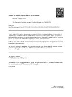
Figure
9
presents a striking demon-
stration of these statements.
It
shows the

path of the sequential sample standard
deviation and the sequential mean abso-
lute deviation for four
se~urities.~' The
upper set of points on each graph repre-
sents the path of the standard deviation,
while the lower set represents the sample
sequential mean absolute deviation. In
40
The mean absolute deviation is defined as
where xis the variable and
N
is the total sample size.
41
Sequential computation of a parameter means
that the
ct~mulative
sequential sample value of the
parameter is recomputed at fixed intervals subse-
quent to the beginning of the sampling period. Each
new computation of the parameter in the sequence
contains the same values of the random variable as
the computation immediately preceding it, plus any
new values of the variable that have since been
generated.
every case the sequential mean absolute
deviation shows less erratic behavior as
the sample size is increased than does the
sequential standard deviation. Even for
very large samples the sequential stand-

ard deviation often shows very large dis-
crete jumps, which are of course due to
the occurrence of extremely large price
changes in the data. As the sample size
is increased, however, these same large
price changes do not have nearly as strong
an effect on the sequential mean absolute
deviation. This would seem to be strong
evidence that for distributions of price
changes the mean absolute deviation is a
much more reliable estimate of variabil-
ity than the standard deviation.
In general, when dealing with stable
Paretian distributions with characteristic
exponents less than
2,
the researcher
should avoid the concept of variance
both in his empirical work and in any
economic models he may construct. For
example, from an empirical point of
view, when there is good reason to believe
that the distribution of residuals has in-
finite variance, it is not very appealing
to use a regression technique that has as
its criterion the minimization of the sum
of squared residuals from the regression
line, since the expectation of that sum
will be infinite.
This does not mean, however, that we

are helpless when trying to estimate the
parameters of a linear model if the vari-
ables of interest are subject to stable
Paretian distributions with infinite vari-
ances. For example, an alternative tech-
nique, absolute-value regression, involves
minimizing the sum of the absolute val-
ues of the residuals from the regression
line. Since the expectation of the absolute
value of the residual will be finite as long
as the characteristic exponent
a
of the
distribution of residuals is greater than
1,
this minimization criterion is meaning-


96
THE
JOURNAL OF BUSINESS
ful for a wide variety of stable Paretian
proce~ses.~~
A
good example of an economic model
which uses the notion of variance in situ-
ations where there is good reason to be-
lieve that variances are infinite is the
classic Markowitz
[39]

analysis of efficient
portfolios. In Markowitz' terms, efficient
portfolios are portfolios which have
max-
42
For a discussion of the technique of absolute
value regression see Wagner
[46], [47].
Wise
[49]
has
shown that when the distribution of residuals has
characteristic exponent
1
<
a
<
2, the usual least
squares estimators of the parameters of a regression
equation are consistent and unbiased. He has further
.085
AMERlCbN
CAN
.020
,
.015:
.
.
.
:.''bhc%~

.010
:
,005
.ooo.
300 600 900 1860
,025
GEN.
MOTORS
.C.20.
.015.
?
\,*A*
,005
.
000
400 800 1200
?
imum expected return for given variance
of expected return.
If
yields on securities
follow distributions kith infinite vari-
ances, however, the expected yield of a
diversified portfolio will also follow a
shown, however, that when
a
<
2, the least squares
estimators are not the most efficient linear esti-
mators, i.e., there are other techniques for which

the sampling distributions of the regression parame-
ters have lower dispersion than the sampling distri-
butions of the least squares estimates. Of course it
is also possible that some non-linear technique, such
as absolute value regression, provides even more
efficient estimates than the most efficient linear
estimators.
.
oes
A.
T.
AND
T.
.020
-
.015
.010.
-
.t:
.005
;.
.,;$
'L 4

-
.w
."O'lj
300 600 900 1200
.095
SEARS

.020.
.015
,
300 600 900 1200
FIG. 9 Sequential standard deviations and sequential mean absolute deviations. Horizontal axes
show sequential sample sizes; vertical axes show parameter estimates.
97
BEHAVIOR OF STOCK-MARKET PRICES
distribution with an infinite variance. In
this situation the mean-variance concept
of an efficient portfolio loses its meaning.
This does
not
mean, however, that
diversification is a meaningless concept
in a stable
Paretian market, or that it is
impossible to develop a model for port-
folio analysis. In a separate paper
[IS]
this author has shown that, if concepts
of variability other than the variance are
used, it is possible to develop a model for
portfolio analysis in a stable
Paretian
market. It is also possible to define the
conditions under which increasing diver-
sification has the effect of reducing the
dispersion of the distribution of the re-
turn on the portfolio, even though the

variance of that distribution may be in-
finite.
Finally, although the Gaussian or nor-
mal distribution does not seem to be an
adequate representation of distributions
of stock price changes, it is not neces-
sarily the case that stable
Paretian dis-
tributions with infinite variances provide
the only alternative.
It
is possible that
there are long-tailed distributions with
finite variances that could also be used to
describe the
data.43 We shall now argue,
however, that one is forced to accept
many of the conclusions discussed above,
regardless of the position taken with re-
spect to the
finite-versus-infinite-vari-
ance argument.
For example, although one may feel
that it is nonsense to talk about infinite
variances when dealing with real-world
variables, one is nevertheless forced to
admit that for distributions of stock price
changes the sampling behavior of the
standard deviation is much more erratic
than that of alternative dispersion

pa-
43
It
is important to note, however, that stable
Paretian distributions with characteristic exponents
less than
2
are the only long-tailed distributions
that have the crucial property of stability or invari-
ance under addition.
rameters such as the mean absolute de-
viation. For this reason it may be better
to use these alternative
dispersion pa-
rameters in empirical work even though
one may feel that in fact all variances
are finite.
Similarly, the asymptotic properties
of the parameters in a classical
least-
squares regression analysis are strongly
dependent on the assumption of finite
variance in the distribution of the resid-
uals. Thus, if in some practical situation
one feels that this distribution, though
long-tailed, has finite variance, in prin-
ciple one may feel justified in using the
least-squares technique.
If,
however, one

observes that the sampling behavior of
the parameter estimates produced by the
least-squares technique is much more
erratic than that of some alternative
technique, one may be forced to conclude
that for reasons of efficiency the alterna-
tive technique is superior to least squares.
The same sort of argument can be
applied to the portfolio-analysis problem.
Although one may feel that in principle
real-world distributions of returns must
have finite variances, it is well known
that the usual Markowitz-type efficient
set analysis is highly sensitive to the
estimates of the variances that are used.
Thus, if it is difficult to develop good
estimates of variances because of erratic
sampling behavior induced by long-tailed
distributions of returns, one may feel
forced to use an alternative measure of
dispersion in portfolio analyses.
Finally, from the point of view of the
individual investor, the name that the
researcher gives to the probability dis-
tribution of the return on a security is
irrelevant, as is the argument concerning
whether variances are finite or infinite.
The investor's sole interest is in the
shape
of the distribution. That is, the only in-

formation he needs concerns the proba-
98
THE JOURNAL OF BUSINESS
bility of gains and losses greater than
given amounts. As long as two different
hypotheses provide adequate descriptions
of the relative frequencies, the investor
is indifferent as to whether the researcher
tells him that distributions of returns are
stable
Paretian with characteristic expo-
nent
a
<
2 or just long-tailed but with
finite variances.
In essence, all of the above arguments
merely say that, given the long-tailed
empirical frequency distributions that
have been observed, in most cases one's
subsequent behavior in light of these
results will be the same whether one leans
toward the Mandelbrot hypothesis or to-
ward some alternative hypothesis involv-
ing other long-tailed distributions. For
most purposes the implications of the
empirical work reported in this paper are
independent of any conclusions concern-
ing the name of the hypothesis which the
data seem to support.

E.
POSSIBLE
DIRECTIONS
FOR
FUTURE
RESEARCH
It
seems safe to say that this paper
has presented strong and voluminous
evidence in favor of the random-walk
hypothesis. In business and economic re-
search, however, one can never claim to
have established a hypothesis beyond
question. There are always additional
tests
which would tend either to confirm
the validity of the hypothesis or to con-
tradict results previously obtained. In
the final paragraphs of this paper we
wish to suggest some possible directions
which future research on the
random-
walk hypothesis could take.
1.
ADDITIONAL
POSSIBLE
TESTS
OF
DEPENDENCE
There are two different approaches to

testing for independence. First, one can
carry out purely statistical tests.
If
these
tend to support the assumption of inde-
pendence, one may then infer that there
are probably no mechanical trading rules
based on patterns in the past history of
price changes which will make the profits
of the investor greater than they would
be under a buy-and-hold policy. Second,
one can proceed by directly testing dif-
ferent mechanical trading rules to see
whether or not they do provide profits
greater than buy-and-hold. The
serial-
correlation model and runs tests dis-
cussed in Section
V
are representative of
the first approach, while Alexander's fil-
ter technique is representative of the
second.
Academic research to date has tended
to concentrate on the statistical ap-
proach. This is true, for example, of the
extremely sophisticated work of Granger
and Morgenstern
[19], Moore
[41],

Ken-
dall[26], and others. Aside from Alexan-
der's work
[I],
[2], there has really been
very little effort by academic people to
test directly the various chartist theories
that are popular in the financial world.
Systematic validation or invalidation of
these theories would represent a real
contribution.
2.
POSSIBLE
RESEARCH
ON
THE
DISTRI-
BUTION
OF
PRICE CHANGES
There are two possible courses which
future research on the distribution of
price changes could take.
First, until now
most research has been concerned with
simply finding statistical distributions
that seem to coincide with the empirical
distributions of price changes. There has
been relatively little effort spent in ex-
ploring the more basic processes that give

rise to the empirical distributions. In
essence, there is as yet no general model
of price formation in the stock market
which explains price levels and distribu-
tions of price changes in terms of the