Báo cáo y học: "A scaling normalization method for differential expression analysis of RNA-seq data" pps
Bạn đang xem bản rút gọn của tài liệu. Xem và tải ngay bản đầy đủ của tài liệu tại đây (654.79 KB, 9 trang )
METH O D Open Access
A scaling normalization method for differential
expression analysis of RNA-seq data
Mark D Robinson
1,2*
, Alicia Oshlack
1*
Abstract
The fine detail provided by sequencing-based transcriptome surveys suggests that RNA-seq is likely to become the
platform of choice for interrogating steady state RNA. In order to discover biologically important changes in
expression, we show that normalization continues to be an essential step in the analysis. We outline a simp le and
effective method for performing normalization and show dramatically improved results for inferring differential
expression in simulated and publicly available data sets.
Background
The transcriptional architecture is a complex and
dynamic aspect of a cell’ s func tion. Next generation
sequencing of steady state RNA (RNA-seq) gives unpre-
cedented detail about the RNA landscape within a cell.
Not only can expression levels of genes be interrogated
without specific prior knowledge, but comparisons of
expression levels between genes within a sample can be
made. It has also been demonstrated that splicing var-
iants [1,2] and single nucleotide polymorphisms [3] can
be detected through sequencing the transcriptome,
opening up the opportunity to interrogate allele-specific
expression and RNA editing.
An important aspect of dealing with the vast amounts
of data generated from short read sequencing is the pro-
cessing methods used to extract and interpret the infor-
mation. Experience with microarray data has repeatedly
shown that normalization is a critical comp onent of the
processing pipeline, allowing accurate estimation and
detection of differential expression (DE) [4]. The aim of
normalization is to remove systematic technical effects
that occur in the data to ensure that technical bias has
minimal impact on the results. However, the pro cedure
for generating RNA-seq data is fundamentally different
from that for microarray data, so the normalization
methods used are not directly applicable. It has been
suggested that ‘ One particularly powerful advantage of
RNA-seq is that it can capture transcriptome dynamics
across different tissues or conditions without
sophisticated normalization of data sets’ [5]. We demon-
strate here t hat the reality of RNA-seq data analysis is
not this simple; normalization is often still an important
consideration.
Current RNA-seq analysis methods typically standar-
dize data between samples by scaling the number of
readsinagivenlaneorlibrarytoacommonvalue
across all sequenced libraries in the experiment. For
example, several authors have modeled the observed
counts for a gene with a mean that includes a factor for
the total number of reads [6-8]. These approaches can
differ in the distrib utional assumptions made for infer-
ring differences, but the consensus is to use the total
number of reads in the model. Similarly, for LONG-
SAGE-seq data, ‘tHoenet al. [9] use the squar e root of
scaled counts or the beta-binomial model of Vencio et
al. [10], bo th of which use the total number of observed
tags. For normalization, Mortazavi et al.[11]adjust
their counts to reads per kilobase per million mapped
(RPKM), suggesting it ‘facilitates transparent comparison
of transcript levels both within and between samples.’ By
contrast, Cloonan et al. [12] log-transform the ge ne
length-normalized count data and apply standard micro-
array analysis techniques (quantile normalization and
moderated t-statistics). Sultan et al. [ 2] normalize read
counts by the ‘virtual length’ of the gene, the number of
unique 27-mers in exonic sequence, as well as by the
total number of reads. Recently, Balwierz et al. [13] illu-
strated that deepCAGE (deep sequ encing cap analysis of
gene expression) data follow an approximate power law
distribution and proposed a normalization strategy that
equates the read count distributions across samples.
* Correspondence: ;
1
Bioinformatics Division, Walter and Eliza Hall Institute, 1G Royal Parade,
Parkville 3052, Australia
Robinson and Oshlack Genome Biology 2010, 11:R25
/>© 2010 Robinson and Oshlack; licensee BioMed Central Ltd. This is an open access article distributed under the terms of the Creative
Commons Attribution License ( which permits unrestricted use, distribution, and
reprodu ction in any medium, provided the original work is properly cited.
Scaling to library size as a form of n ormalization
makes intuitive sense, givenitisexpectedthatsequen-
cing a sample to half the depth will give, o n average,
half the number of reads mapping to each gene. We
believe this is appropriate for normalizing between repli-
cate samples of an RNA population. However, library
size scaling is too simple for many biological applica-
tions. The number of tags expecte d to map to a ge ne is
not only dependent on the expression level and length
of the gene, but also the composition of the RNA popu-
lation that is being sampled. Thus, if a large number of
genes are unique to, or highly expressed in, one experi-
mental condition, the sequencing ‘real estate’ available
for the remaining genes in tha t sample is decreased. If
not adjusted for, this sampling artifact can force the DE
analysis to be skewed towards one experimental condi-
tion. Current analysis methods [6,11] have not
accounted for this proportionality property of the data
explicitly, potentially giving rise to hi gher false positive
rates and lower power to detect true differences.
The fundamental issue here is the appropriate metric
of expression to compare across samples. The standard
procedure is to compute the proportion of each gene’ s
reads relative to the total number of reads and compare
that across all samples, either by transforming the origi-
nal data or by introducing a constant into a statistical
model. However, since different experimental conditions
(for example, tissues) express diverse RNA repertoires,
we cannot always expect the proportions to be directly
comparable. Furthermore, we argue that in the discovery
of biologically meaningful changes in expression, it
should be considered undesirable to have under- or
oversampling effects (discussed further below) guiding
the DE calls. The normalization method presented
below uses the raw data to estimate appropriate scaling
factors that can be used in downstream statistical analy-
sis procedures, thus accounting for the sampling proper-
ties of RNA-seq data.
Results and discussion
A hypothetical scenario
Estimated normalization factors should ensure that a
gene with the same expression level in two samples is
not detected as DE. To further highlight the n eed for
more sophisticated normalization procedures in RNA-
seq data, consider a simple thought experiment. Imagine
we have a sequencing experiment comparing two RNA
populations, A and B. In this hypothetical scenario, sup-
pose every gene that is expressed in B is expressed in A
with the same number of transcripts. However, assume
that sample A also contains a set of genes equal in
number and expression that are not expressed in B.
Thus, sample A has twice as many total expressed genes
as sample B, that is, its RNA production is twice the
size of sample B. Suppose that each sample is then
sequenced to the same depth. Without any additional
adjustment, a gene expressed in both samp les will have,
on average, half the number of reads from sample A,
since the reads are spread over twice as many genes.
Therefore, the correct normalization would adjust sam-
ple A by a factor of 2.
The hypothetical example above highlights the notion
that the p roportion of reads attributed to a given gene
in a library depends on the expression properties of the
whole sample rather than just the expression level of
that gene. Obviously, the above example is artificial.
However, there are biological and even technical situa-
tions where such a normalization is required. For exam-
ple, if an RNA sample is contaminated, the reads that
represent the contamination will take away reads from
the true sample, thus dropping the number of reads of
interest and offsetting the proportion for every gene.
However, as we demonstrate, true biological differences
in RNA composition between samples will be the main
reason for normalization.
Sampling framework
A more formal explanatio n for t he requirement of nor-
malization uses the following framework. Define Y
gk
as
the observed count for gene g in library k summarized
from the raw reads, μ
gk
asthetrueandunknown
expression level (number of transcripts), L
g
as the length
of gene g and N
k
as total number of reads for library k.
We can model the expected value of Y
gk
as:
EY
gk
L
g
S
k
N
SL
gk k
kgkg
g
G
[]
;
where
1
S
k
represents the total RNA output of a sample. The
problem underlying the analysis of RNA-seq data is that
while N
k
is known, S
k
is unknown and can vary drasti-
cally from sample to sample, depending on the RNA
compositio n. As mentione d above, if a population has a
larger total RNA output, then RNA-seq experiments will
under-sample many genes, relative to another sample.
At this stage, we leave the variance in the above
model for Y
gk
unspecified. Depending on the experimen-
tal situation, Poisson seems appropriate for technical
replicates [6,7] and Negative Binomial may be appropri-
ate for the additio nal variation observed from biological
replicates [14]. It is also worth noting that, in practice,
the L
g
is generally absorbed into the μ
gk
parameter and
does not get used in the inference procedure. However,
it has been well established that gene length biases are
prominent in the analysis of gene expression [15].
Robinson and Oshlack Genome Biology 2010, 11:R25
/>Page 2 of 9
The trimmed mean of M-values normalization method
The total RNA production, S
k
, cannot be estimated
directly, since we do not know the expression levels and
true lengths of every gene. However, the relative RNA
production of two samples, f
k
=S
k
/S
k’
, essentially a glo-
bal fold change, can more easily be determined. We pro-
pose an empirical strategy that equates the overall
expression levels of genes between samples under the
assumption that t he majority of them are not DE. One
simple yet robust way to estimate the ratio of RNA pro-
duction uses a weighted trimmed mean of the log
expression ratios (trimmed mean of M values (TMM)).
For sequencing data, we define the gene-wise log-fold-
changes as:
M
Y
gk
N
k
Y
gk
N
k
g
log
/
/
2
and absolute expression levels:
AYNYNY
ggkkgkkg
1
2
0
2
log
’
for
To robustly summarize the observed M values, we
trim both the M values and the A values before taking
the weighted average. Precision (inverse of the variance)
weights are used to account for the fact that log fold
changes (effectively, a log relative risk) from genes with
larger read counts have lower variance on the logarithm
scale. See Materials and methods for further details.
For a two -sample comparison, only one relative scal-
ing factor (f
k
) is required. It can be used to adjust both
library sizes (divide the reference b y
f
k
and multiply
non-reference by
f
k
) in the statistical analysis (for
example, Fisher’s exact test; see Materials and methods
for more details).
Normalization factors across several samples can be
calculated by selecting one sample as a reference and
calculating the TMM factor for each non-reference
sample. Similar to two-sample comparisons, the TMM
normalization factors can be built into the statistical
model used to t est for DE. For example, a P oisson
model would modify the observed library size to an
effective library size, which adjusts the modeled mean
(for example, using an additional offset in a generalized
linear model; see Materials and methods for further
details).
A liver versus kidney data set
We applied our method to a publicly available transcrip-
tional profiling data set comparing several technical
replicates of a liver and kidney RNA source [6]. Figure
1a shows the distribution of M values between two tech-
nical replicates of the kidney sample after the standard
normalization procedure of ac counting for the total
number of reads. The distribution of M values for these
technical replicates is concentrated around zero. How-
ever, Figure 1b shows that log ratios between a liver and
kidney sample are significantly offset towards higher
expression in kidney, even after accounting for the total
number of reads. Also highlighted (green line) is the dis-
tribution of observed M values for a set of housekeeping
genes, showing a significant shift away from zero. If
scaling to the total numbe r of reads appropriately nor-
malized RNA-seq data, then such a shift in the log-fold-
changes is not expected. The explanation for this bias is
straightforward. The M versus A plot in Figure 1c illus-
trates that there exists a prominent set of genes with
higher expression in liver (black arrow). As a result, the
distribution of M values (liver to kidney) is skewed in
the negative direction. Since a large amount of sequen-
cing is dedicated to these liver-specific genes, there is
less sequencing available for the remaining genes, thus
proportionally distorting the M values (and therefore,
the DE calls) towards being kidney-specific.
The application of TMM normalization to this pair of
samples results in a normalization factor of 0.68 (-0.56
onlog2scale;shownbytheredlineinFigure1b,c),
reflecting the under-sampling of the majority of liver
genes. The TMM factor is robust for lower coverage
data where more genes with zero counts may b e
expected (Figure S1a in Additional f ile 1) and is stable
for reasonable values of the trim parameters (Figure S1b
in Additional file 1). Using TMM normalization in a sta-
tistical test for DE (see Materials and methods) results
in a similar number of genes significantly higher in liver
(47%) and kidney (53%). By contrast, the standard nor-
malization (to the total number of reads as originally
used in [6]) result s in the majority of DE genes being
significantly higher in kidney(77%).Notably,lessthan
70% of the genes identified as DE using standard nor-
malization are still detected after TMM normalization
(Table 1). In addition, we find the log-fold-changes for a
large set of housekeeping genes (from [16]) are, on aver-
age, offset from zero very close to the estimated TMM
factor, thus g iving credibility to our robust estimation
procedure. Furthermore, using the non-adjusted testing
procedure, 8% and 70% of the housekeeping genes are
significantly up-regulated in liver and kidney, respec-
tively. After TMM adjustment, the proportion of DE
housekeeping genes changes to 26% and 41%, respec-
tively, which is a lower total number and more sym-
metric between the two tissues. Of course, the bias in
log-ratios observed in RNA-seq data is not observed in
microarray data (from the same sources of RNA),
assuming the microarray data have been appropriately
normalized (Figure S2 in Additional file 1). Taken
together, these results indicate a critical role for the nor-
malization of RNA-seq data.
Robinson and Oshlack Genome Biology 2010, 11:R25
/>Page 3 of 9
Other datasets
The global shift in log-fold-change caused by RNA com-
position differences occurs at varying degrees in other
RNA-seq datasets. For example, an M versus A plot for
the Cloonan et al. [12] dataset (Figure S3 in Additional
file 1) gives an estimated TMM scaling factor of 1.04
between the two samples (embryoid bodies versus
embryonic stem cells), sequenced on the SOLiD™ sys-
tem. The M versus A plot for this dataset also highlights
an interesting set of genes that have lower overall
expression, but higher in embryoid bodies. This explains
the positive shift in log-fold-changes for t he remaining
genes. The TMM scale factor appears close to the med-
ian log-fold-changes amongst a set of approximately 500
mouse housekeeping genes (from [17]). As another
example, the Li et al. [18] dataset, using the llumina 1G
Genome Analyzer, exhibits a shift in the overall distri-
bution of log-fold-changes and gives a TMM scaling fac-
tor of 0.904 (Figure S4 in Additional file 1). However,
there are sequencing-based datasets that have quite
similar RNA outputs and may not need a significant
adjustment. For example, the small-RNA-seq data from
Kuchenbauer et al. [19] exhibits only a modest bias in
the log-fold-changes (Figure S5 in Additional file 1).
Spike-in controls have the potential to be used for
normalization. In this scenario, small but known
amounts of RNA from a foreign organism are added to
each sample at a specified concentration. In order to
use spike-in controls for normalization, the ratio of the
concentration of the spike to the sample must be kept
constant throughout the experiment. In practice, this is
difficult to achieve and small variations will lead to
biased estimation of the normalization factor. For exam-
ple, using the spiked-in DNA from the Mortazavi et al.
data set [11] would lead to unrealistic normalization fac-
tor estimates (Figure S6 in Additional file 1). As with
Figure 1 Normalization is required for RNA-seq data. Data from [6] comparing log ratios of (a) technical replicates and (b) liver versus
kidney expression levels, after adjusting for the total number of reads in each sample. The green line shows the smoothed distribution of log-
fold-changes of the housekeeping genes. (c) An M versus A plot comparing liver and kidney shows a clear offset from zero. Green points
indicate 545 housekeeping genes, while the green line signifies the median log-ratio of the housekeeping genes. The red line shows the
estimated TMM normalization factor. The smear of orange points highlights the genes that were observed in only one of the liver or kidney
tissues. The black arrow highlights the set of prominent genes that are largely attributable for the overall bias in log-fold-changes.
Table 1 Number of genes called differentially expressed
between liver and kidney at a false discovery rate <0.001
using different normalization methods
Library size
normalization
TMM
normalization
Overlap
Higher in liver 2,355 4,293 2,355
Higher in
kidney
8,332 4,935 4,935
Total 10,867 9,228 7,290
House keeping
genes (545)
Higher in liver 45 137 45
Higher in
kidney
376 220 220
Total 421 357 265
TMM, trimmed mean of M values.
Robinson and Oshlack Genome Biology 2010, 11:R25
/>Page 4 of 9
microarrays, it is generally more robust to carefully esti-
mate normalization factors using the experimental data
(for example, [20]).
Simulation studies
To investigate the range in util ity of the TMM normali-
zation method, we developed a simulation framework to
study the effects of RNA composition on DE analysi s of
RNA-seq data. To start, we simulate data from just two
libraries. We include parameters for the number of
genes expressed uniquely to each sample, and para-
meters for the proportion, magnitude and direction of
differentially expressed genes between samples (see
Material and methods). Figure 2a shows an M versus A
plot for a typ ical simulation including unique genes and
DE genes. By simulating different total RNA outputs,
the majority of non-DE genes have log-fold-changes that
are offset from zero. In this case, using T MM normali-
zation to account for the underlying RNA composition
leads to a lower number of false detections using a Fish-
er’ s exact test (Figure 2b). Repeating the simulat ion a
large number of times across a wide range of simulation
parameters, we find good agreement when comparing
the true normalization factors from the simulation with
those estimated using TMM normalization (Figure S7 in
Additional file 1).
To further compare the performance of the TMM
normalization with previously used methods in the con-
text of the DE analysis of R NA-seq data, we extend the
above simulation to include replicate sequencing runs.
Specifically, we compare three published methods:
length-normalized count data that have b een log tra ns-
formed and quantile normalized, as implemented by
Cloonan et al. [12], a Poisson regression [6] with library
size and TMM normalization and a Poisson exact test
[8] with library size and TMM normalization. We do
not compare directly with the normalization proposed
in Balwierz et al. [13] since the liver and kidney dataset
do not appear to follow a power law distribution and
have quite distinct count distributions (Figure S8 in
Additional file 1). Furthermore, in light of the RNA
composition bias we observe, i t is not clear whether
equating the count distributions across sample s is the
most logical procedure. In addition, we do not directly
compare the normalization to virtual length [2] or
RPKM [11] normalization, since a statistical analysis of
the transformed data was not ment ioned. However, we
illustrate with M versus A plots that their normalization
does not completely remove RNA composition bias
(Figures S9 and S10 in Additional file 1).
For the simulation, we used an empirical joint distri-
bution of gene lengths and counts, since the Cloonan
Figure 2 Simulations sho w TMM normalization is robust and outperforms libr ary size normalization. (a) An example of the simulation
results showing the need for normalization due to genes expressed uniquely in one sample (orange dots) and asymmetric DE (blue dots). (b) A
lower false positive rate is observed using TMM normalization compared with standard normalization.
Robinson and Oshlack Genome Biology 2010, 11:R25
/>Page 5 of 9
et al. procedure requires both. We made the simul ation
data Poisson-distributed to mimic technical replicates
(Figure S11 in Additional file 1). Figure 3a shows false
discovery plots amongst the genes that a re common to
both conditions, where we have introduced 10% unique-
to-group expression for the first condition, 5% DE at a
2-fold level, 80% of which is higher in the first condi-
tion. The approach that uses methodology developed for
microarray data performs uniformly worse, as one might
expect since the distributional assumptions for these
methods are quite different. Among the r emaining
methods (Poisson likelihood ratio statistic, Poisson exact
statistic), performance is very similar; again, the TMM
normalization makes a dramatic improvement to both.
Conclusions
TMM normalization is a simple and effective method
for e stimating relative RNA production level s from
RNA-seq data. The TMM method estimates scale fac-
tors between samples that can be incorporated into cur-
rently used statistical methods for DE analysis. We have
shown that normalization is required in situations
where the underlying distribution of expressed tran-
scripts between samples is markedly different. The
assumptions behind the TMM method are similar to
the assumptions commonly made in microarray normal-
ization procedures such as lowess normalization [21]
and quantile normalization [22]. Therefore, adequately
normalized array data do not show the effects of differ-
ent total RNA output between samples. In essence, both
microarray and TMM normalization assume that the
majority of genes, common to both samples, are not dif-
ferentially expressed. Our s imulation studies indicate
that the TMM method is robust against deviations to
this assumption up to about 30% of DE in one direc-
tion. For many applications, this assumption will not be
violated.
One notable difference with TMM normalization for
RNA-seq is that the data themselves do not need to be
modified, unlike microarray normalization and some
implemented RNA-seq strategies [11,12]. Here, the
estimated normalization factors are used directly in the
statistical model used to test for DE, while preserving
the sampling properties of the data. Because the data
Figure 3 False discovery pl ots comparing several publi shed methods.Theredlinedepictsthelength-normalizedmoderatedt-statistic
analysis. The solid and dashed lines show the library size normalized and TMM normalized Poisson model analysis, respectively. The blue and
black lines represent the LR test and exact test, respectively. It can be seen that the use of TMM normalization results in a much lower false
discovery rate.
Robinson and Oshlack Genome Biology 2010, 11:R25
/>Page 6 of 9
themselves are not modified, it can be used in further
applications such as comparing expression between
genes.
Normalization will be crucial in many other applica-
tions of high throughput sequencing where the DNA or
RNA populations being compared differ in their compo-
sition. For example, chromatin immunoprecipitation
(ChIP) followed by next generation sequencing (ChIP-
seq) may require a similar adjustment to compare
between samples containing diffe rent repertoires of
bound targets. Interestingly, the PeakSeq method [23]
uses a linear regression on binned counts across the
genome to estimate a scaling factor between two ChIP
populations to account for the different coverages. This
is similar in principle to what is proposed here, but pos-
sibly less robust. We demonstrated that there are
numerous biological situations where a composition
adjustment will be required. In addition, technical arti-
facts that are not fully captured by the library size
adjustment can be accounted for with the empirical
adjustment. Furthermore, it is not clear that DNA
spiked-in at known concentrations will allow robust
estimation of normalization factors.
Similar to previous high throughput technologies such
as microarrays, normalization is an essential step for
inferring true differences in expression between samples.
The number of reads for a gene is dependent not only
on the gene’s expression level and length, but a lso on
the population of RNA from which it originates. We
present a straightforward and effective empirical method
for normalization of RNA-seq data.
Materials and methods
TMM normalization details
A trimmed mean is the average after removing the
upper and lower x% of the data. The TMM procedure is
doubly trimmed, by log-fold-changes
M
gk
r
(sample k
relative to sample r for gene g) and by absolute intensity
(A
g
). By default, we trim the M
g
values by 30% and the
A
g
values by 5%, but these settings can be tailored to a
given experiment. The software also allows the user to
set a lower bound on the A value, for instances such as
the Cloonan et al. dataset (Figure S1 in Additional file
1). After trimming, we take a weighted mean of M
g
,
with weights as the inverse of the approximate asympto-
tic variances (calculated using the delta method [24]).
Specifically, the normalization factor for sample k using
reference sample r is calculated as:
log ( )
*
*
log
()
2
2
TMM
w
gk
r
M
gk
r
gG
w
gk
r
gG
M
Y
gk
N
k
k
r
gk
r
where
log
;
,
2
Y
gr
N
r
w
N
k
Y
gk
N
k
Y
gk
N
r
Y
gr
N
r
Y
gr
Y
gk
r
gk
and
YY
gr
0.
The cases where Y
gk
=0orY
gr
= 0 are trimmed in
advance of this calculation since log-fold-changes cannot
be calculated; G* represents the set of genes with valid
M
g
and A
g
values and not trimmed, using t he percen-
tages above. It should be clear that
TMM
r
r()
1
.
As Figure 2a indicates, the variances of the M values
at higher total count are lower. Within a library, the
vector of counts is multinomial distributed and any indi-
vidual gene is binomial distributed with a given library
size and proportion. Using t he delta method, one can
calculate an approximate variance for the M
g
,asiscom-
monly done with log relative risk, and the inverse of
these is used to weight the average.
We compared the weighted with the unweighted
trimmed mean as well as an alternati ve robust estimator
(robust linear model) over a range of simulation para-
meters, as shown in Figure S4 in Additional file 1.
Housekeeping genes
Human housekeeping genes, as described in [16], were
downloaded from [25] and matched to the Ensembl gene
identifiers using the Bioconductor [26] biomaRt package
[27]. Similarly, mouse housekeeping genes were taken to
be the approximately 500 genes with lowest coefficient of
variation, as calculated by de Jonge et al. [17].
Statistical testing
For a two-library comparison, we use the sage.test func-
tion from the CRAN statmod package [ 28] to calculate
aFisherexactP-value for each gene. To apply TMM
normalization, we replace the original library sizes with
‘effective’ library sizes. For two libraries, the effective
library sizes are calculated by multiplying/dividing the
square root of the estimated normalization factor with
the original library size.
For comparisons with technical replicates, we followed
the analysis procedure used in the Marioni et al. study
[6]. Briefly, it is assumed that the counts mapping to a
gene are Poisson-distributed, according to:
YPoisM
gk gz k
k
~( )
where
gz
k
represents the fraction of total reads for
gene g in experimental condition z
k
. Their analysis utilizes
an offset to account for the library size and a likelihood
ratio (LR) stat istic to test for differences in expression
between libraries (that is, H
0
:μ
g1
= μ
g2
). In order to use
TMM normalization, we augment the original offset with
the estimated normalization factor. The same LR testing
framework is then used to calculate P-values for DE
between tissues. We modified this analysis to use an exact
Poisson test for testing the difference between two
Robinson and Oshlack Genome Biology 2010, 11:R25
/>Page 7 of 9
replicated groups. The strategy is similar in principle to
the Fisher’s exact test: conditioning on the total count, we
calculated the probability of observing group counts as or
more extreme than what we actually observed. Th e total
and group total counts are all Poisson distributed.
We re-implemented the method from Cloonan et al.
[12] for the analysis of simul ated data using a custom R
[29] script.
Simulation details
The simulation is set up to sample a dataset from a
given empirical distribution of read counts (that is, from
a distribution of observed Y
g
). The mean is calculated
from the sampled read counts divided by the sum S
k
and multiplied by a specified library size N
k
(according
to the model). The simulated data are then randomly
sampled from a Poisson distribution, given the mean.
We have parameters specifying the number of genes
common to both libraries and the number of genes
unique to each sample. Additi onal parameters specify
the amount, direction and magnitude of DE as well as
the depth of sequencing (that is, range of total number s
of reads). Since we have inserted known differentially
expressed genes, we can rank genes according to various
statistics and plot the number of false discoveries as a
function of the ranking. Table S1 in Additional file 1
gives the parameter settings used for the simulations
presented in Figures 2 and 3.
Software
Sof tware implementing our method was released within
the edgeR package [30] in version 2.5 of Bioconductor
[26] and is available from [31]. Scripts and data for our
analyses, including the simulation framework, have been
made available from [32].
Additional file 1: A Word document with supplementary materials,
including 11 supplementary figures and one supplementar y table.
Click here for file
[ />r25-S1.doc ]
Abbreviations
ChIP: chromatin immunoprecipation; DE: differential expression; LR:
likelihood ratio; RPKM: reads per kilobase per million mapped; TMM:
trimmed mean of M values.
Acknowledgements
We wish to thank Terry Speed, Gordon Smyth and Matthew Wakefield for
helpful discussion and critical reading of the manuscript. This work is partly
supported by the National Health and Medical Research Council (481347-
MDR, 490037-AO)
Author details
1
Bioinformatics Division, Walter and Eliza Hall Institute, 1G Royal Parade,
Parkville 3052, Australia.
2
Epigenetics Laboratory, Cancer Program, Garvan
Institute of Medical Research, 384 Victoria Street, Darlinghurst, NSW 2010,
Australia.
Authors’ contributions
MDR and AO conceived of the idea, analyzed the data and wrote the paper.
Received: 19 November 2009 Revised: 28 January 2010
Accepted: 2 March 2010 Published: 2 March 2010
References
1. Wang ET, Sandberg R, Luo S, Khrebtukova I, Zhang L, Mayr C, Kingsmore SF,
Schroth GP, Burge CB: Alternative isoform regulation in human tissue
transcriptomes. Nature 2008, 456:470-476.
2. Sultan M, Schulz MH, Richard H, Magen A, Klingenhoff A, Scherf M,
Seifert M, Borodina T, Soldatov A, Parkhomchuk D, Schmidt D, O’Keeffe S,
Haas S, Vingron M, Lehrach H, Yaspo ML: A global view of gene activity
and alternative splicing by deep sequencing of the human
transcriptome. Science 2008, 321:956-960.
3. Wang X, Sun Q, McGrath SD, Mardis ER, Soloway PD, Clark AG:
Transcriptome-wide identification of novel imprinted genes in neonatal
mouse brain. PLoS One 2008, 3:e3839.
4. Bolstad BM, Irizarry RA, Astrand M, Speed TP: A comparison of
normalization methods for high density oligonucleotide array data
based on variance and bias. Bioinformatics 2003, 19:185-193.
5. Wang Z, Gerstein M, Snyder M: RNA-Seq: a revolutionary tool for
transcriptomics. Nat Rev Genet 2009, 10:57-63.
6. Marioni JC, Mason CE, Mane SM, Stephens M, Gilad Y: RNA-seq: an
assessment of technical reproducibility and comparison with gene
expression arrays. Genome Res 2008, 18:1509-1517.
7. Bullard JH, Purdom EA, Hansen KD, Durinck S, Dudoit S: Statistical
inference in mRNA-Seq: exploratory data analysis and differential
expression. UC Berkeley Division of Biostatistics Working Paper Series 2009,
paper 247.
8. Robinson MD, Smyth GK: Small-sample estimation of negative binomial
dispersion, with applications to SAGE data. Biostatistics 2008, 9:321-332.
9. t Hoen PA, Ariyurek Y, Thygesen HH, Vreugdenhil E, Vossen RH, de
Menezes RX, Boer JM, van Ommen GJ, den Dunnen JT: Deep sequencing-
based expression analysis shows major advances in robustness,
resolution and inter-lab portability over five microarray platforms. Nucleic
Acids Res 2008, 36:e141.
10. Vencio RZ, Brentani H, Patrao DF, Pereira CA: Bayesian model accounting
for within-class biological variability in serial analysis of gene expression
(SAGE). BMC Bioinformatics 2004, 5:119.
11. Mortazavi A, Williams BA, McCue K, Schaeffer L, Wold B: Mapping and
quantifying mammalian transcriptomes by RNA-Seq. Nat Methods 2008,
5:621-628.
12. Cloonan N, Forrest AR, Kolle G, Gardiner BB, Faulkner GJ, Brown MK,
Taylor DF, Steptoe AL, Wani S, Bethel G, Robertson AJ, Perkins AC, Bruce SJ,
Lee CC, Ranade SS, Peckham HE, Manning JM, McKernan KJ, Grimmond SM:
Stem cell transcriptome profiling via massive-scale mRNA sequencing.
Nat Methods 2008, 5:613-619.
13. Balwierz PJ, Carninci P, Daub CO, Kawai J, Hayashizaki Y, Van Belle W,
Beisel C, van Nimwegen E: Methods for analyzing deep sequencing
expression data: constructing the human and mouse promoterome with
deepCAGE data. Genome Biol 2009, 10:R79.
14. Robinson MD, Smyth GK: Moderated statistical tests for assessing
differences in tag abundance. Bioinformatics 2007, 23:2881-2887.
15. Oshlack A, Wakefield MJ: Transcript length bias in RNA-seq data
confounds systems biology. Biol Direct 2009, 4:14.
16. Eisenberg E, Levanon EY: Human housekeeping genes are compact.
Trends Genet 2003, 19:362-365.
17. de Jonge HJ, Fehrmann RS, de Bont ES, Hofstra RM, Gerbens F, Kamps WA,
de Vries EG, Zee van der AG, te Meerman GJ, ter Elst A: Evidence based
selection of housekeeping genes. PLoS One 2007, 2:e898.
18. Li H, Lovci MT, Kwon YS, Rosenfeld MG, Fu XD, Yeo GW: Determination of
tag density required for digital transcriptome analysis: application to an
androgen-sensitive prostate cancer model. Proc Natl Acad Sci USA 2008,
105:20179-20184.
19. Kuchenbauer F, Morin RD, Argiropoulos B, Petriv OI, Griffith M, Heuser M,
Yung E, Piper J, Delaney A, Prabhu AL, Zhao Y, McDonald H, Zeng T,
Robinson and Oshlack Genome Biology 2010, 11:R25
/>Page 8 of 9
Hirst M, Hansen CL, Marra MA, Humphries RK: In-depth characterization of
the microRNA transcriptome in a leukemia progression model. Genome
Res 2008, 18:1787-1797.
20. Oshlack A, Emslie D, Corcoran LM, Smyth GK: Normalization of boutique
two-color microarrays with a high proportion of differentially expressed
probes. Genome Biol 2007, 8:R2.
21. Yang YH, Dudoit S, Luu P, Lin DM, Peng V, Ngai J, Speed TP: Normalization
for cDNA microarray data: a robust composite method addressing single
and multiple slide systematic variation. Nucleic Acids Res 2002, 30:e15.
22. Irizarry RA, Hobbs B, Collin F, Beazer-Barclay YD, Antonellis KJ, Scherf U,
Speed TP: Exploration, normalization, and summaries of high density
oligonucleotide array probe level data. Biostatistics 2003, 4:249-264.
23. Rozowsky J, Euskirchen G, Auerbach RK, Zhang ZD, Gibson T, Bjornson R,
Carriero N, Snyder M, Gerstein MB: PeakSeq enables systematic scoring of
ChIP-seq experiments relative to controls. Nat Biotechnol 2009, 27:66-75.
24. Casella G, Berger RL: Statistical Inference Pacific Grove, CA: Duxbury Press
2002.
25. Housekeeping Genes. [ />Housekeeping_genes.html].
26. Gentleman RC, Carey VJ, Bates DM, Bolstad B, Dettling M, Dudoit S, Ellis B,
Gautier L, Ge Y, Gentry J, Hornik K, Hothorn T, Huber W, Iacus S, Irizarry R,
Leisch F, Li C, Maechler M, Rossini AJ, Sawitzki G, Smith C, Smyth G,
Tierney L, Yang JY, Zhang J: Bioconductor: open software development
for computational biology and bioinformatics. Genome Biol 2004, 5:R80.
27. Durinck SMY, Kasprzyk A, Davis S, De Moor B, Brazma A, Huber W: BioMart
and Bioconductor: a powerful link between biological databases and
microarray data analysis. Bioinformatics 2005, 21:3439-3440.
28. CRAN - Package statmod. [ />index.html].
29. Team RDC: R: A Language and Environment for Statistical Computing 2009.
30. Robinson MD, McCarthy DJ, Smyth GK: edgeR: a Bioconductor package
for differential expression analysis of digital gene expression data.
Bioinformatics 2010, 26:139-140.
31. Bioconductor. [ />32. WEHI Bioinformatics - Resources. [ />doi:10.1186/gb-2010-11-3-r25
Cite this article as: Robinson and Oshlack: A scaling normalization
method for differential expression analysis of RNA-seq data. Genome
Biology 2010 11:R25.
Submit your next manuscript to BioMed Central
and take full advantage of:
• Convenient online submission
• Thorough peer review
• No space constraints or color figure charges
• Immediate publication on acceptance
• Inclusion in PubMed, CAS, Scopus and Google Scholar
• Research which is freely available for redistribution
Submit your manuscript at
www.biomedcentral.com/submit
Robinson and Oshlack Genome Biology 2010, 11:R25
/>Page 9 of 9