Báo cáo y học: "Modeling non-uniformity in short-read rates in RNA-Seq data" ppt
Bạn đang xem bản rút gọn của tài liệu. Xem và tải ngay bản đầy đủ của tài liệu tại đây (1.62 MB, 11 trang )
Li et al. Genome Biology 2010, 11:R50
/>Open Access
METHOD
© 2010 Li et al.; licensee BioMed Central Ltd. This is an open access article distributed under the terms of the Creative Commons Attri-
bution License ( which permits unrestricted use, distribution, and reproduction in any
medium, provided the original work is properly cited.
Method
Modeling non-uniformity in short-read rates in
RNA-Seq data
Jun Li
1
, Hui Jiang
1,2
and Wing Hung Wong*
1,3
Modeling RNA-seq dataMethods for modeling read counts from short read RNA-seq data.
Abstract
After mapping, RNA-Seq data can be summarized by a sequence of read counts commonly modeled as Poisson
variables with constant rates along each transcript, which actually fit data poorly. We suggest using variable rates for
different positions, and propose two models to predict these rates based on local sequences. These models explain
more than 50% of the variations and can lead to improved estimates of gene and isoform expressions for both Illumina
and Applied Biosystems data.
Background
Microarrays are an efficient technology to measure the
expression levels of many genes simultaneously, but there
are some limitations to this method. The expression esti-
mates are typically not reliable for lowly expressed genes
because the true signals are masked by cross-hybridiza-
tion effects [1,2]. Furthermore, the design of the array
depends on annotation of gene structures and thus the
method is not ideal for the discovery of novel splicing
events. A recently developed alternative approach, called
RNA-Seq, has the potential to overcome these difficulties
[3]. RNA-Seq uses ultra-high-throughput sequencing [4]
to determine the sequence of a large number of cDNA
fragments. The resulting sequences (reads) can be long
(>100 nucleotides) or short, depending on the platform
[4]. Two currently popular short-read platforms are Illu-
mina's Solexa [5-11] and Applied Biosystems' (ABI's)
SOLiD [12]. Each can produce tens of millions of short
reads in a single run [5-12]. In this paper, we only con-
sider the short-read RNA-Seq.
The reads produced by RNA-Seq are first mapped to
the genome and/or to the reference transcripts using
computer programs. Then, the output of RNA-Seq can be
summarized by a sequence of 'counts'. That is, for each
position in the genome or on a putative transcript, it gives
a count standing for the number of reads whose mapping
starts at that position. As an example (we have shortened
the gene and reads for simplification), if a gene with a sin-
gle isoform has sequence ACGTCCCC, and we have 12
ACGTC reads, 8 CGTCC reads, 9 GTCCC reads, and 5
TCCCC reads, then this gene can be summarized by a
sequence of counts 12, 8, 9, 5.
Quantitative inference of RNA-Seq data, such as calcu-
lating gene expression levels [7] and isoform expression
levels [13], is based on these counts. To utilize the data
efficiently, it is crucial to have an appropriate statistical
model for these counts. Current analysis methods
assume, explicitly or implicitly, a naive constant-rate Pois-
son model, in which all counts from the same isoform are
independently sampled from a Poisson distribution with
a single rate proportional to the expression level of the
isoform [7,13,14]. Unfortunately, we found that this
model does not provide a good fit to real data (see
Results), and a more elaborate model is needed.
To better model the counts, it is natural to consider a
Poisson model with variable rates; that is, the counts
from an isoform are still modeled as Poisson random
variables, but each Poisson random variable has a differ-
ent rate (mean value). By checking the similarities among
counts of different tissues (see Results), one can see that
the Poisson rate depends on not only the gene expression
level, but also the position of the read. Hence, we model
the rate as the product of the gene expression level and
the 'sequencing preference' of reads starting at this posi-
tion. This sequencing preference is a factor showing how
likely it is for a read to be generated at this position.
Dohm et al. [15] found that GC-rich regions tend to
have more reads than AT-rich regions, but we find that
models based purely on GC content work poorly (Addi-
tional file 1). Some clues on how to model the sequencing
* Correspondence:
1
Department of Statistics, Stanford University, Sequoia Hall, 390 Serra Mall,
Stanford, CA 94305, USA
Full list of author information is available at the end of the article
Li et al. Genome Biology 2010, 11:R50
/>Page 2 of 11
preferences may be obtained by reviewing how related
issues are handled in microarrays. There are a set of
probes for each gene in microarrays, and each probe gives
a continuous measurement of the gene expression level.
The values of the measurements from the same set are
modeled by a Gaussian distribution with different means,
each of which is the product of the gene expression level
and the affinity of that probe to the cDNA sequences.
Naef and Magnasco [16] proposed a model for the probe
affinities, which only depends on the probe sequences:
where ω
i
is the affinity of probe i, K is the length of the
probe, I(b
ik
= h)) is 1 when the k
th
base pair is letter h, and
0 otherwise, α and β
kh
are the parameters we want to esti-
mate, and ε is Gaussian noise so that the parameters can
be estimated by regular linear least squares. The key fea-
ture of this model is that it considers the letter appearing
at each location, rather than just the total number of
occurrences of each letter. This simple linear model can
explain 44% of the differences of the affinities in an
Affymetrix oligonuleotide array dataset. Similar models
have been developed for other arrays or datasets [17-20].
In RNA-Seq experiments, cDNA synthesis is typically
initiated by random priming. Depending on its sequence,
an mRNA fragment may form secondary structures that
obstruct the binding of the primers. Furthermore, the
primer is usually tagged by a non-random flanking
sequence that may preferentially interact with the mRNA
depending on the mRNA sequence. Due to these effects,
the probability for binding depends on both the nucle-
otide sequence and the protocol. After synthesis, the
cDNAs are ligated to linkers, amplified and then
sequenced. In these steps, the secondary structure of the
cDNA and the details of the protocol can again influence
the efficiency. Therefore, the protocol and the local
sequence context may have a large influence on how
likely an mRNA segment will be read. Hence, under a
specific protocol, we may be able to predict, at least
partly, the sequencing preferences based on the local
nucleotide sequences.
Results and discussion
Datasets and overdispersion
Three genome-wide RNA-Seq datasets are used in this
paper. The first two were generated by Illumina's Solexa
platform, and the third one was generated by ABI's
SOLiD platform. The first dataset [7] is composed of 79,
76, and 70 million reads from three mouse tissues: brain,
liver and skeletal muscle. Each read is of length 25. The
second dataset [11] is composed of 12 to 29 million reads
from 10 diverse human tissues and 5 mammary epithelial
or breast cancer cell lines. Each read is of length 32. We
use data from nine of these tissues or cell lines, and merge
them into three groups (adipose, brain, and breast in
group one, colon, heart, and liver in group two, lymph
node, skeletal muscle, and testes in group three.). Each
group contains 61 to 77 million reads. The third dataset
[12] is composed of 16 million high-quality reads from
each of the two cell lines: embryoid bodies (EB) and
undifferentiated mouse embryonic stem cells (ES). Each
original read is 35 nucleotides, but some are truncated
into 30 or 25 nucleotides to ensure high quality. We refer
to these three datasets as Wold data, Burge data, and
Grimmond data, respectively, in accord with the research
group that originally generated the data. As we just
described, each of the three datasets contains several sub-
datasets standing for different tissues, groups, or cell
lines, and in total we have eight sub-datasets: three (tis-
sues) for Wold data, three (groups) for Burge data, and
two (cell lines) for Grimmond data. In all our processing
and calculations, the above sub-datasets are considered
separately; that is, only one sub-dataset is analyzed at a
time.
First, the count data are extracted from the original
datasets. The detailed procedure is described in Materials
and methods. Briefly speaking, we map reads to all iso-
forms of all RefSeq genes, and then in order to avoid
ambiguity, we only count reads uniquely mapped to genes
that have only one isoform annotated in RefSeq and do
not overlap with other genes, which we call 'non-over-
lapped single-transcript genes'. Further, we use only the
counts from the top 100 genes with the highest expres-
sion levels to fit our model since they have the highest
signal-to-noise ratio (see Additional file 1 for details).
Two pieces of evidence clearly show that the counts
violate the Poisson model with a constant rate. First, the
data are seriously overdispersed. A basic property of Pois-
son distribution is the equality of mean and variance. If
variance is larger than mean, then the data are said to be
overdispersed, and the Poisson assumption is inappropri-
ate. Table 1 lists the maximum, median, and minimum
values of the variance-to-mean ratios (also called 'Fano
factor') in the top 100 genes of each sub-dataset. All the
ratios are much larger than 1. Second, the 'pattern' (rela-
tive values) of counts across a gene is surprisingly con-
served in different sub-datasets of the same dataset.
Figure 1 shows the counts in the gene Apoe (apolipopro-
tein E) of all three tissues of the Wold data. Although the
absolute values of the counts varies by 100-fold in differ-
ent tissues, the patterns of variation are highly consistent
across tissues. The same holds true in other genes of the
Wold data and in genes of the Burge and Grimmond data.
This is strong evidence that the counts for different posi-
tions from the same gene are not sampled from the same
log( ) ( )
{,,}
wa b e
ikhik
hACGk
K
Ib h=+ = +
∈=
∑∑
1
Li et al. Genome Biology 2010, 11:R50
/>Page 3 of 11
distribution. Rather, the distribution of a count seems to
depend on the position of its sequence in the transcript.
This compels us to consider more sophisticated models.
The observation that the biases in read rates are strongly
dependent on local sequences has also been described by
Hansen et al. [21], which is an independent work that
came to our attention when our paper was under review.
The Poisson linear model and its performance
For nucleotide j of gene i, we want to model how the dis-
tribution of the count of reads starting at this nucleotide
(denoted as n
ij
) depends on the expression level of this
gene (denoted as μ
i
) and the nucleotide sequence sur-
rounding this nucleotide (the sequence with length K is
denoted as b
ij1
, b
ij2
, , b
ijK
,). We assume n
ij
~Poisson (μ
ij
),
where μ
ij
is the rate of the Poisson distribution, and μ
ij
=
ω
ij
μ
i
, where ω
ij
is the sequencing preference, which may
depend on the surrounding sequence. As a simple
approach, we use a linear model for the preference and
hence the Poisson rate:
where ν
i
= log(μ
i
), α is a constant term, I(b
ijk
= h) equals
to 1 if the k
th
nucleotide of the surrounding sequence is h,
and 0 otherwise, and β
kh
is the coefficient of the effect of
letter h occurring in the k
th
position. This model uses
about 3K parameters to model the sequencing preference.
To fit the above model, we iteratively optimize the gene
expression levels and the Poisson regression coefficients
(Materials and methods).
We applied our model to each of the eight sub-datasets.
As local sequence context, we use 40 nucleotides prior to
the first nucleotide of the reads and 40 nucleotides after
them (that is, the first 40 nucleotides of the reads; see
Additional file 1 for the reason for choosing this region).
Thus, our model uses 3 × 80 = 240 parameters to model
the sequencing preference. This is a relatively small num-
log( ) ( )
{,,}
mna b
ij i kh ijk
hACGk
K
Ib h=++ =
∈=
∑∑
1
Figure 1 Counts of reads along gene Apoe in different tissues of
the Wold data. (a) Brain, (b) liver, (c) skeletal muscle. Each vertical line
stands for the count of reads starting at that position. The grey lines are
counts in the UTR regions and a further 100 bp. Here introns are delet-
ed and exons are connected into a single piece. Only shown are counts
on one strand of the gene; counts on the other strand show similar
similarities in different tissues. Nt: nucleotides.
0 400 800 12000 2000 4000 6000
0 200 400 600 800 1000 1200
(c)
(b)
(a)
position (nt)
count
0
20 40 60 80
Table 1: Variance-to-mean ratios in different datasets
Variance-to-mean ratios
Dataset Sub-dataset Maximum Median Minimum
Wold Brain 248 36 21
Liver 1,503 48 19
Muscle 2,088 34 18
Burge Group 1 835 78 14
Group 2 1,187 102 28
Group 3 1,593 112 20
Grimmond EB 24,385 806 47
ES 9,162 345 22
Li et al. Genome Biology 2010, 11:R50
/>Page 4 of 11
ber compared to the sample size (about 100,000 counts)
in each sub-dataset.
In linear regression, the percentage of variance that can
be explained by the regression, denoted by R
2
, is used to
measure the goodness-of-fit. In Poisson regression, we
can replace variance by deviance and define:
where d is the deviance of the fitted model, and d
0
is the
deviance of the null model [22]. In our case, the null
model is the naive model assuming the same sequencing
preference. The final R
2
values we achieved are listed in
Table 2. Roughly speaking, this simple linear model can
explain about 40 to 50% of the variance.
Figure 2 shows all coefficients in the linear model. The
asymptotic standard error of each coefficient is approxi-
mately 0.002, so almost all coefficients are statistically
very significant. This is not surprising, as our sample size
is much bigger than the number of parameters. In this
case, what are more important are the magnitudes of the
coefficients. Generally, the coefficients in the central part
of the figure have larger absolute values than those on
both sides, where they approach zero. This shows that the
nucleotides around the first position of a read have
greater effect on the sequencing preference. This is rea-
sonable, as these nucleotides tend to form with the head
of a read local secondary structure, which involves only
several nucleotides and is thus easy to predict. Although
farther nucleotides may form non-local secondary struc-
ture with the head of a read, it is hard to predict the struc-
ture since it involves too many nucleotides and may differ
dramatically from case to case.
The coefficients are strikingly similar in each sub-data-
set of the same dataset, although they significantly differ
in different datasets. This is strong evidence that these
coefficients are meaningful rather than just random.
Although it is difficult to explain biologically the mag-
nitude of each coefficient, it is possible for us to explain
the main differences of coefficients between datasets by
the protocols they used. Both the Wold and Burge data
were generated by using the Illumina platform, so their
curves look similar, especially in the central part. How-
ever, the mRNAs were fragmented into approximately
200-nucleotide pieces before cDNA synthesis in the Wold
data but not in the Burge data. Shorter pieces of mRNA
are less likely to form non-local secondary structure.
Therefore, the coefficient curve of the Wold data should
have lighter tails. Grimmond's experiment used ABI's
platform for sequencing and added quite different linkers
to the synthesized cDNA before sequencing, so the whole
curve looks quite different from that of the Wold and
Burge data.
Our Poisson linear model shows that at least 37 to 52%
of the non-uniformity can be explained by the sequence
difference. However, this percentage may be an underes-
timate of the fraction of deviance explainable by local
sequence context as the simple linear model cannot cap-
ture many other effects. Adding more predictors to the
linear model is possible, and in particular adding the
dinucleotide composition can considerably improve the
Rdd
2
1=−/
0
Table 2: R
2
in different datasets
R
2
Poisson linear MART
Dataset Sub-dataset 80 nucleotides
a
,
non-cross-validation
80 nucleotides
a
,
cross-validation
40 nucleotides
a
,
cross-validation
40 nucleotides
a
,
cross-validation
Wold Brain 0.52 0.51 0.51 0.70
Liver 0.51 0.50 0.50 0.70
Muscle 0.48 0.46 0.46 0.59
Burge Group 1 0.43 0.42 0.42 0.52
Group 2 0.37 0.35 0.35 0.46
Group 3 0.45 0.42 0.42 0.54
Grimmond EB 0.47 0.40 0.40 0.58
ES 0.45 0.39 0.37 0.54
a
The lengths of the surrounding sequences we consider.
Li et al. Genome Biology 2010, 11:R50
/>Page 5 of 11
fitting (Additional file 1), but we prefer to consider non-
linear models to get a better understanding of how much
of the non-uniformity of the counts is systematic bias
rather than random noise.
The MART model and its performance
Having tried methods such as support vector machines
and neural networks (Additional file 1), we settled on
MART (multiple additive regression trees) as our final
choice for a nonlinear model. MART is a gradient tree-
boosting algorithm proposed by Friedman [23,24]. One
version of MART is available in the 'gbm' package [25] of
R [26]. Also, to avoid the over-fitting that commonly
occurs for nonlinear models, we use cross-validation and
R
2
in the testing data.
The details on using MART and on estimating cross-
validation R
2
are given in Materials and methods. In this
analysis, we use shorter surrounding sequences. For the
Wold and Burge data, we use 25 nucleotides prior to the
first nucleotide of the reads and 15 nucleotides after it,
and for the Grimmond data, we use 15 nucleotides prior
and 25 nucleotides after. These are the regions that have
large coefficients in the Poisson regression model (Addi-
tional file 1). Using shorter surrounding sequences lowers
the dimensions of the input data, thus shortening the
training time and reducing the chance of over-fitting.
The final cross-validation R
2
values we achieved are
listed in Table 2. Seven out of eight R
2
values are larger
than 0.50, and two of them are as high as 0.70. Compared
with the linear model, R
2
increases by 0.10 to 0.20, show-
ing the power of the MART model. Figure 3 gives us an
illustrative example of how our two methods perform.
Figure 3a-c shows the counts on gene Apoe in the original
data, counts fitted by the Poisson linear model, and
counts fitted by MART, respectively. It is easy to see that
MART fits the counts much better. For this reason, we
suggest that the MART model should be used when we
make any statistical inferences from the data, while the
Poisson linear model is only used to select a reasonable
region of surrounding sequences for MART. We also note
that the fitted counts determined using MART change
more quickly along the gene than those determined using
the Poisson linear model, but in neither case are the
changes as drastic as in the original data. Actually, the
variance-to-mean ratios of fitted counts by the two meth-
ods are 55 and 91, both less than 127, the ratio in the orig-
inal counts. This indicates that both of our models still
give conservative fits.
Our high R
2
shows that at least 50 to 70% of the non-
uniformity in the sequencing preference is predictable
from local sequences.
The model we trained using the most-highly expressed
genes can be used to predict the sequencing preference
for other genes. As an example, we predicted for the brain
sample of the Wold data the preferences for all unique
genes using the MART model trained using the top 100
genes only, and the results are summarized by R
2
(Figure
4). As expected, R
2
is smaller for genes with lower expres-
sion levels, since unpredictable randomness accounts for
Figure 2 The coefficients of the Poisson linear models in different
datasets. The coefficients of the Poisson linear model in the eight sub-
datasets when we consider surrounding sequences as 40 nucleotides
before and 40 nucleotides after the first nucleotide of a read. Position -
1, 0, 1 means the nucleotide before the first nucleotide of a read, the
first nucleotide of a read, and the second nucleotide of a read, respec-
tively. Color coding for nucleotides: red, T; green, A; blue, C; black, G.
The coefficients for nucleotide T (red) are the base levels, so they are
always zero. (a) Coefficients in the Wold data. Shape coding for sub-
datasets: rectangle, brain; triangle, liver; circle, skeletal muscle. (b) Co-
efficients in the Burge data. Shape coding for sub-datasets: rectangle,
group 1; triangle, group 2; circle, group 3. (c) Coefficients in the Grim-
mond data. Shape coding for sub-datasets: rectangle, EB; triangle, ES.
Following are examples of how these coefficients should be read. In
the Wold brain data, the coefficient of C in the first nucleotide of a read
(the blue rectangle at position 0 in (a)) is 0.82. This means that if the nu-
cleotide T is replaced by C, then the sequencing preference will in-
crease to e
0.82
= 2.27 times. Nt: nucleotides.
-1.5
(b)
(c)
-1.0 -0.5 0.0 0.5
(a)
coefficients
-1.0 -0.5 0.0 0.5-1.0 -0.5 0.0 0.5
-40 -30 -20 -10 0 10 20 30 40
position (nt)
Li et al. Genome Biology 2010, 11:R50
/>Page 6 of 11
a larger portion of variability in a Poisson distribution
with a small mean. The average R
2
is above 0.5 for high or
moderately expressed genes (the reads per kilobase of
exon per million mapped sequence reads (RPKM) >30),
and no R
2
for genes with RPKM >1 is negative, indicating
our model performs consistently better than the uniform
model. Note that in these data, 1 RPKM stands for only
0.034 reads per nucleotide on average.
Applications of our models
Our results may benefit quantitative inference from
RNA-Seq data. To reduce biases in gene expression esti-
mates due to non-uniformity of read rates, we propose to
estimate the expression of a single-isoform gene by the
total number of reads along the gene divided by the sum
of sequencing preferences (SSP) under our MART model.
In contrast, the standard estimate will divide the number
of reads by the length of the gene, which is equivalent to
dividing by the SSP under the uniform model where all
sequencing preferences are set to be 1.
To test the new method, we first compared the gene
expression levels estimated using the mouse liver sub-
dataset of the Wold RNA-Seq data with those estimated
using Affymetrix microarray data of the same tissue, as
used by Kapur et al. [27]. For RNA-Seq data, we estimate
gene expression level under the uniform model and our
MART model, and for microarray data, we use the
Robust Multichip Average [28]. All non-overlapped sin-
gle-transcript genes are included in the comparison, and
the results are summarized by the Spearman's rank corre-
lation coefficients. For all genes considered, using our
MART model increased the rank correlation from 0.771
to 0.773 compared to the uniform model, which repre-
sents a very minor improvement.
What is the reason for the failure of our highly predic-
tive model for sequencing preferences to lead to more
significant improvements in gene expression estimates?
We believe the answer is that when a gene is large, the
dramatic local variations in the sequencing preferences
will be smoothed out when they are summed over many
positions to produce the SSP for the whole gene. In this
case the SSP under the MART model will not be very dif-
ferent from the SSP under the uniform model, and the
new estimate will be almost the same as the usual esti-
mate. To see whether the new estimate can lead to
improvement in those cases when it is different from the
standard estimate, we first quantify the difference
between the two estimates by their fold-change, defined
as:
Figure 3 Fitting counts for the Apoe gene. Black vertical lines repre-
sent counts (experimental values or fitted values) along the Apoe gene
(with the UTR and a further 100 nucleotides truncated). (a) Counts of
reads (true values) in the Wold brain data. This is the same as the cen-
tral part (black vertical lines) of Figure 1a. (b) Counts of fitted reads us-
ing the Poisson linear model. We use the other 99 genes of the top 100
genes to train the linear model, which is then used to predict the
counts for Apoe. This prediction has a (cross-validation) R
2
= 0.54. (c)
Counts of fitted reads using MART. We use the other 99 genes of the
top 100 genes to train MART, which is then used to predict the counts
for Apoe. This prediction has a (cross-validation) R
2
= 0.69.
0
200 400 600 800
0 200 400 600 800
0 200 400 600
0 200 400 600 800
count
(a)
(b)
(c)
position (nt)
Figure 4 Boxplot of R
2
for unique genes in the Wold brain data.
We divided the genes with at least one read into six groups according
to their RPKMs: <1, 1 to 5, 5 to 15, 15 to 30, 30 to 100, and >100; each
group contains 4,205, 3,320, 2,807, 1,330, 1,094, and 383 genes, respec-
tively. Note that in these data, 1 RPKM stands for 0.034 reads per nucle-
otide on average, a gene with RPKM >30 is considered to be relatively
abundant, and a gene with RPKM <1 is not robust even for transcript
detection [7].
RPKM
R
2
<1 1~5 5~15 15~30 30~100 >100
-0.4 -0.2 0.0 0.2 0.4 0.6 0.8
Li et al. Genome Biology 2010, 11:R50
/>Page 7 of 11
The average fold change across genes in the Wold data
is only 1.02; thus, it is not surprising that the performance
of the new estimate is so close to the standard estimate.
Consistently, when we examine the 100 genes with the
largest fold changes (on average, the fold change is 1.10 in
these 100 genes), the rank correlation shows a much
larger improvement, from 0.095 to 0.198, that is, a 108%
relative change.
Table 3 presents the average fold changes of genes,
exons and junctions of chromosome 1 for the different
data sets. We see that the fold change can be substantially
larger than 1 depending on how large the region is over
which we are averaging the sequencing preferences, the
sequencing platform, and the lab that generated the data.
For example, the Grimmond data show an average fold
change of 1.25 across genes. We thus expect the new esti-
mate will show a greater improvement for this data. To
see if this is the case, we note that Kapur et al. [27] calcu-
lated the gene expression levels of the Affymetrix
microarray data from mouse embryo samples, which we
can use to assess the new estimate and the standard esti-
mate for the Grimmond EB data. For all genes consid-
ered, the rank correlation coefficient increases from 0.439
for the standard estimate to 0.469 for the new estimate, a
6.9% relative change. We further classified the genes into
five bins according to their fold change of SSP, each con-
taining about 20% of all genes. Table 4 shows the rank
correlation coefficients of gene expression levels for
genes in each bin. It is very clear that bigger improve-
ments occur in genes with larger fold changes. For the
20% of genes whose fold changes are the smallest, the
improvement is only about 0.1%, but for the 20% of genes
whose fold changes are the largest, the improvement is
about 26%. Most significantly, for the 100 genes whose
fold changes are the largest, the rank correlation changes
from 0.323 to 0.526, a 62.8% relative improvement. These
results show that our new estimate based on modeling
sequencing preferences can lead to significant improve-
ments in gene expression estimates.
Next we examined whether incorporation of sequenc-
ing preferences can lead to improved inferences for iso-
form-specific expression levels. We modified the
isoform-specific expression estimates in Jiang et al. [13]
by assuming the mean count for each exon to be propor-
tional to the SSP of the exon instead of the length of the
exon. Figure 5 shows the four isoforms of the RefSeq gene
Clta in mouse. Under the uniform model, the method in
[13] gives isoform expression of 21.6%, 53.4%, 8.95%, and
16.0% (let the sum to be 100%) for the Grimmond EB
data. When the sequencing preferences are taken into
account, the method in [13] gives 15.5%, 52.9%, 10.8%,
and 20.7%. The new counts based on the new expression
levels and sequence preferences fit the data much better
(data not shown).
Returning to the Wold data, we note from Table 3 that
the fold change for SSP for exons is 1.12, which suggests
the possibility that there may be enough differences in the
exon-level estimates between the MART model and the
uniform model. To assess the performance of the two
models with regard to exon-level estimates, we compared
our estimates of the isoform expression levels with those
given in Pan et al. [29], who studied 3,126 'cassette-type'
alternative splicing (AS) events in 10 mouse tissues using
custom microarrays. Every AS event in each tissue was
targeted by seven probes, and then a percent alternatively
spliced exon exclusion value (%ASex) was computed as a
summary statistic. In the paper by Jiang et al. [13], which
introduced their method for estimating isoform expres-
sion levels, they compared %ASex by Pan et al. [29] with
%ASex calculated based on the uniform model for three
mouse tissues: liver, muscle and brain. In particular, they
selected subsets of the AS events based on two criteria:
one requires a moderate expression level of the gene and
a relatively narrow confidence interval of the %ASex; and
the other additionally requires a moderate percentage of
the exon-excluded isoform. We used the same subsets of
genes, taking the sequencing preferences predicted by
MART into account, and used their approach to calculate
%ASex. The results are summarized in Table 5. For
almost every subset of genes, the Pearson's correlation
coefficients are higher when we consider sequencing
fo d change
under MART under uniform
u
l =
max( , )
min(
SSP SSP
SSP
nnder MART under uniform,)SSP
Table 3: Average fold changes of genes, exons, and junctions of chromosome 1
Average fold changes of mean sequencing preferences
Dataset used to train
the model
Genes Exons Junctions (read
length = 35)
Junctions (read
length = 100)
Wold 1.02 1.12 1.13 1.07
Burge 1.181.321.371.28
Grimmond 1.25 2.17 2.34 1.73
Li et al. Genome Biology 2010, 11:R50
/>Page 8 of 11
preferences, and the average relative improvement is
about 7.2%. This suggests that our MART model offers
meaningful improvement for the isoform expression level
estimate even for the Wold data, which has the least
amount of non-uniformity.
In the above, we find that the main factor determining
how much improvement our model can bring is the mag-
nitude of fold changes. Thus, we expect that our method
can be applied to many other problems that involve short
sequence elements. In new isoform discovery, a problem
of great current interest, it is crucial to take into account
the relative counts of reads along the region. For example,
a region with more reads per base than its surrounding
regions suggests a new exon. However, this might be mis-
leading if this region has more reads merely because it
has larger sequencing preferences than its surrounding
regions. Further effort is needed to incorporate our
method into current isoform-discovery algorithms.
While the MART model gives better estimates of
sequencing preferences and is thus used for statistical
inference, the main purpose of the Poisson linear model
is to select a proper K for the MART model. Neverthe-
less, it might still be possible for us to get more informa-
tion from it, especially from the plot of the coefficients
(like Figure 2). For example, if the coefficients in the cen-
tral part of the curve have large absolute values, this may
indicate that the difference in sequencing preferences is
repeatedly enlarged in the experiment, most likely by
multi-round PCR, and we may need to use more mRNA
samples instead of doing PCR for too many rounds. As
another example, if the coefficient curve has heavy tails,
this should indicate that the mRNA/cDNA tend to form
complex non-local secondary structure, which is also
unfavorable, and we may need to fragment the mRNAs
into smaller pieces and/or choose better linkers with
proper lengths. It might be possible for experienced tech-
nicians, who know all the details of the experiments, to
provide more explanation of, or even pinpoint, the main
causes of biases. This might help to improve the proto-
cols of RNA-Seq.
Conclusions
Non-uniformity is dramatic in RNA-Seq data
In each of the eight sub-datasets, the RNA-Seq count data
are largely over-dispersed. This is strong evidence that
the non-uniformity of the counts is too great for Poisson
distribution with constant rate tocapture. Also, among
the sub-datasets of each dataset, the trends that counts
differ along the gene show a highly consistent pattern.
This is not only evidence that the Poisson distribution
fails, but also suggests that the changes of the counts
depend on the position along the gene.
Table 4: Spearman's rank correlation coefficients in mouse embryoid bodies
Fold change bin SCC by uniform model SCC by our MART model Relative improvement
(1.00, 1.09) 0.465 0.466 0.1%
(1.09, 1.19) 0.437 0.444 1.4%
(1.19, 1.33) 0.413 0.434 5.1%
(1.33, 1.53) 0.481 0.520 8.2%
(1.53, 4.82) 0.389 0.490 26.0%
SCC: Spearman's rank correlation coefficient.
Figure 5 Four isoforms of RefSeq gene Clta in mouse. This figure was generated using the CisGenome browser [36]. At the top are shown the base
positions in mouse chromosome 4 and exons as grey blocks. On the bottom are shown the four isoforms, with exons zoomed in. The tail of exon 1 of
the first isoform is 6 bp less than that of the other three isoforms. The second isoform has 7 exons, while the third isoform misses both exon 5 (54 bp)
and exon 6 (36 bp), and the fourth isoform misses exon 6.
44026000 44030000 44034000 44038000
44042000
NM_001080386
NM_001080385
NM_001080384
NM_016760
Li et al. Genome Biology 2010, 11:R50
/>Page 9 of 11
Poisson linear model
We proposed a Poisson linear model for the count data,
and implement an iterative Poisson linear regression pro-
cedure to fit it. Using the surrounding 80 nucleotides, it is
able to explain 37 to 52% of the difference in the counts
for the most highly expressed genes. We find that the
coefficients for nucleotides near the first nucleotide of a
read have bigger abstract values, indicating that they play
a more important role in determining the sequencing
preferences.
MART model
To capture the nonlinear effects of the local sequences,
we use MART to fit the log preferences, and a cross-vali-
dation strategy is implemented to calculate R
2
. MART
gives a cross-validation R
2
of 0.52 to 0.70 in seven out of
eight sub-datasets, a 0.10 to 0.20 improvement. This
result indicates that the major information about non-
uniformity is in the local sequences.
Benefits of our models
Our models may help us to evaluate the protocol for
RNA-Seq experiments. It can also give us better estima-
tors for the quantitative inferences of RNA-Seq data.
Since the average preferences can vary substantially in
short pieces of sequences, the improvement can be signif-
icant. We believe that all quantitative analysis of RNA-
Seq data should incorporate sequencing preference infor-
mation. Particularly, we suggest training a model for
sequencing preference using only the top 100 genes and
MART, then using this trained model to predict the
sequencing preference of all sites in the transcriptome,
which are then used in further inferences.
Materials and methods
Extracting the count data from the original reads data
First, we downloaded from the UCSC genome browser
website [30] the sequences of RefSeq genes [31,32]
(mouse July 2007 mm9 for the Wold and Grimmond data,
and human Feb 2009 hg19 for the Burge data). Then, we
mapped the reads to all isoforms of the RefSeq genes. For
Illumina data, we directly mapped the 25 or 32 nucleotide
reads using SeqMap [33], allowing two mismatches. For
ABI data, we used the same strategy as described in Sup-
plementary Figure 1 of [12], where a three-round map-
ping for 35, 30 and 25 nucleotide qualified reads was
performed separately. In each round, we used SOCS [34]
as the mapping tool. After mapping, we selected genes
that have only one isoform annotated in RefSeq and do
not overlap with other genes, and called them 'non-over-
lapped single-isoform genes'. To avoid ambiguity, we only
retained reads that map to a unique site and this site is
within the unique genes. Then, we counted the number
of reads whose mapping starts at each position of these
unique genes, which gives the count data. Since some
positions have the same local sequence (to the length of
reads) as other positions because of the short length of
reads, they are always assigned a zero count by our count-
ing method. This might influence the results of our analy-
sis. However, these positions comprise less than 2% of all
positions even if the read length is only 25, so they should
not change our analysis significantly.
Several more steps are performed afterwards. To avoid
UTR ambiguity in the annotation and boundary bias in
the sequencing [3], we truncated all UTRs and a further
100 nucleotides on both ends. We then discarded genes
that are too short (less than 100 nucleotides) after the
truncation. Finally, after calculating the gene expression
levels measured by RPKM [7], we discarded all genes
except the top 100 with the highest expression levels. The
counts of these top genes were the only counts we used
for fitting the models. Reads from these top genes make
up a considerable proportion of all reads mapped unam-
biguously, and thus give sufficient information for the
sequencing preference. In contrast, lowly expressed genes
have no or only a few reads across them, and moderate-
Table 5: Pearson's correlation coefficients of %A Sex
Selection
criterion
Tissue Number of
selected AS
events
PCC by uniform
model
PCC by our MART
model
Relative
improvement
1 Liver 472 0.48 0.50 4.2%
Muscle 451 0.40 0.45 12.5%
Brain 699 0.36 0.40 11.1%
2Liver 2280.600.600%
Muscle 194 0.48 0.51 6.3%
Brain 298 0.44 0.50 13.6%
PCC: Pearson's correlation coefficient.
Li et al. Genome Biology 2010, 11:R50
/>Page 10 of 11
expressed genes often have zero counts for a considerable
proportion of sites; thus, information on their sequencing
preference is limited.
The count data for the top 100 genes in each sub-data-
set are available in the R package 'mseq' [35], which is
publicly available in CRAN (The Comprehensive R
Archive Network).
Fitting the Poisson linear model
We use the following strategy to fit our Poisson regres-
sion model:
1. Initialize , where L
i
is the length
of gene i.
2. Viewing as known offsets, fit the Poisson
regression model to get and . This is a standard
algorithm, and 'glm()' of R [26] implements it.
3. Update , where W
i
is the sum
of sequencing preferences of all nucleotides of gene i, that
is, .
4. Jump to step 2 unless the deviance decreases less
than 1%.
In the above, step 2 gives the maximum likelihood esti-
mate of α and β
kh
given , and it is easy to prove
that step 3 gives the maximum likelihood estimate of ν
i
given α = and β
kh
= . So the above procedure max-
imizes the likelihood by iteratively optimizing the prefer-
ence parameters and the gene expression levels.
The R codes implementing this procedure are available
in the R package 'mseq' [35].
Strategy for using MART and estimating cross-validation R
2
The strategy for using MART and estimating cross-vali-
dation R
2
includes the following steps: (1) Randomly
divide the 100 genes into 5 groups. In each fold of cross-
validation, use one of them as the testing set, and the
other four as the training set. (2) In each fold, for each
gene in the training dataset, divide each count by the
mean of counts in this gene. The resulting number is con-
sidered to be the sequencing preference of that position.
To avoid zero preference, which is troublesome in step 3,
we replace zero counts by a small number (0.5 in our cal-
culation). (3) Get the logarithm of these preferences. (4)
Train MART using the surrounding sequences as input
and these log preferences as output. The parameters we
used for MART are: interaction depth = 10, shrinkage =
0.06, and number of trees = 2000 (the method is robust to
the choice of parameters; Additional file 1). Also, we put
heavier weights on log preferences from more highly
expressed genes since they have smaller variance. The
weights for log preferences from gene i are set to be N
i
/L
i
,
where N
i
is the total number of reads across this gene, and
L
i
is the length of this gene. (5) Use the trained MART to
predict the log preferences of the testing data. (6) Get the
maximum likelihood estimate of the gene expression lev-
els. That is, suppose for a gene the length is L, the log
preferences are a
1
, , a
L
, and the counts are n
1
, , n
L
, then
the gene expression level is
(7) Calculate the deviance
according to the log preferences in step 5 and the gene
expression levels in step 6. Also calculate the null devi-
ance. (8) Repeat steps 2 to 7 for all five folds. (9) Calculate
the final cross-validation R
2
, which is the sum of devi-
ances in the five folds over the sum of null deviances.
The R codes implementing this procedure are available
in the R package 'mseq' [35].
Additional material
Abbreviations
ABI: Applied Biosystems; Apoe: apolipoprotein E; AS: alternative splicing;
%ASex: percent alternatively spliced exon exclusion; bp: base pair; EB:
embryoid body; ES: embryonic stem cell; MART: multiple additive regression
trees; RPKM: reads per kilobase of exon per million mapped sequence reads;
SSP: sum of sequencing preferences; UTR: untranslated region.
Authors' contributions
JL, HJ and WHW conceived the study. JL developed the methods, performed
the analysis, and drafted the manuscript. HJ and WHW reviewed and revised
the manuscript. All authors have read and approved the final manuscript.
Acknowledgements
This research is supported by NIH grants R01 HG004634 and R01 HG003903.
The computation in this project was performed on a system supported by NSF
computing infrastructure grant DMS-0821823. We thank Xi Chen for discussion
about protocols of RNA-Seq experiments. We also thank three anonymous
reviewers for their insightful and constructive comments and suggestions,
which improved our paper substantially.
Author Details
1
Department of Statistics, Stanford University, Sequoia Hall, 390 Serra Mall,
Stanford, CA 94305, USA,
2
Stanford Genome Technology Center, 855 California
Ave, Palo Alto, CA 94304, USA and
3
Department of Health Research and Policy,
Stanford University, 259 Campus Drive, Redwood Building, Stanford, CA 94305,
USA
n
∧
=
⎡
⎣
⎢
⎢
⎤
⎦
⎥
⎥
=
∑
i
ij
j
L
i
nL
i
log /
1
nn
i
i
=
∧
a
∧
b
∧
kh
n
∧
=
⎡
⎣
⎢
⎢
⎤
⎦
⎥
⎥
=
∑
i
ij
j
L
i
nW
i
log /
1
WIbh
i
kh
ijk
hCTGk
K
j
L
i
=+ =
⎛
⎝
⎜
⎜
⎞
⎠
⎟
⎟
∧∧
∈==
∑∑∑
exp ( )
{,,}
ab
11
nn
i
i
=
∧
a
∧
b
∧
kh
Additional file 1 Supplementary material. Word document containing
supplementary material for this paper, which provides details and discus-
sion about the methods we propose.
Received: 20 November 2009 Revised: 13 April 2010
Accepted: 11 May 2010 Published: 11 May 2010
This article is available from: 2010 Li et al.; licensee BioMed Central Ltd. This is an open access article distributed under the terms of the Creative Commons A ttribution License ( which permits unrestricted use, distribution, and reproduction in any medium, provided the original work is properly cited.Genome Biology 2010, 11:R50
n
=
==
∑∑
na
j
j
L
j
j
L
11
exp( )
Li et al. Genome Biology 2010, 11:R50
/>Page 11 of 11
References
1. Okoniewski MJ, Miller CJ: Hybridization interactions between probesets
in short oligo microarrays lead to spurious correlations. BMC
Bioinformatics 2006, 7:276.
2. Royce TE, Rozowsky JS, Gerstein MB: Toward a universal microarray:
prediction of gene expression through nearest-neighbor probe
sequence identification. Nucleic Acids Res 2007, 35:e99.
3. Wang Z, Gerstein M, Snyder M: RNA-Seq: a revolutionary tool for
transcriptomics. Nat Rev Genet 2009, 10:57-63.
4. Holt RA, Jones SJ: The new paradigm of flow cell sequencing. Genome
Res 2008, 18:839-846.
5. Nagalakshmi U, Wang Z, Waern K, Shou C, Raha D, Gerstein M, Snyder M:
The transcriptional landscape of the yeast genome defined by RNA
sequencing. Science 2008, 320:1344-1349.
6. Wilhelm BT, Marguerat S, Watt S, Schubert F, Wood V, Goodhead I, Penkett
CJ, Rogers J, Bahler J: Dynamic repertoire of a eukaryotic transcriptome
surveyed at single-nucleotide resolution. Nature 2008, 453:1239-1243.
7. Mortazavi A, Williams BA, McCue K, Schaeffer L, Wold B: Mapping and
quantifying mammalian transcriptomes by RNA-Seq. Nat Methods
2008, 5:621-628.
8. Lister R, O'Malley RC, Tonti-Filippini J, Gregory BD, Berry CC, Millar AH,
Ecker JR: Highly integrated single-base resolution maps of the
epigenome in Arabidopsis. Cell 2008, 133:523-536.
9. Marioni JC, Mason CE, Mane SM, Stephens M, Gilad Y: RNA-seq: an
assessment of technical reproducibility and comparison with gene
expression arrays. Genome Res 2008, 18:1509-1517.
10. Morin R, Bainbridge M, Fejes A, Hirst M, Krzywinski M, Pugh T, McDonald
H, Varhol R, Jones S, Marra M: Profiling the HeLa S3 transcriptome using
randomly primed cDNA and massively parallel short-read sequencing.
Biotechniques 2008, 45:81-94.
11. Wang ET, Sandberg R, Luo S, Khrebtukova I, Zhang L, Mayr C, Kingsmore
SF, Schroth GP, Burge CB: Alternative isoform regulation in human
tissue transcriptomes. Nature 2008, 456:470-476.
12. Cloonan N, Forrest AR, Kolle G, Gardiner BB, Faulkner GJ, Brown MK, Taylor
DF, Steptoe AL, Wani S, Bethel G, Robertson AJ, Perkins AC, Bruce SJ, Lee
CC, Ranade SS, Peckham HE, Manning JM, McKernan KJ, Grimmond SM:
Stem cell transcriptome profiling via massive-scale mRNA sequencing.
Nat Methods 2008, 5:613-619.
13. Jiang H, Wong WH: Statistical inferences for isoform expression in RNA-
Seq. Bioinformatics 2009, 25:1026-1032.
14. Pan Q, Shai O, Lee LJ, Frey BJ, Blencowe BJ: Deep surveying of alternative
splicing complexity in the human transcriptome by high-throughput
sequencing. Nat Genet 2008, 40:1413-1415.
15. Dohm JC, Lottaz C, Borodina T, Himmelbauer H: Substantial biases in
ultra-short read data sets from high-throughput DNA sequencing.
Nucleic Acids Res 2008, 36:e105.
16. Naef F, Magnasco MO: Solving the riddle of the bright mismatches:
labeling and effective binding in oligonucleotide arrays. Phys Rev E Stat
Nonlin Soft Matter Phys 2003, 68:011906.
17. Johnson WE, Li W, Meyer CA, Gottardo R, Carroll JS, Brown M, Liu XS:
Model-based analysis of tiling-arrays for ChIP-chip. Proc Natl Acad Sci
USA 2006, 103:12457-12462.
18. Potter DP, Yan P, Huang TH, Lin S: Probe signal correction for differential
methylation hybridization experiments. BMC Bioinformatics 2008, 9:453.
19. Wu ZJ, Irizarry RA, Gentleman R, Martinez-Murillo F, Spencer F: A model-
based background adjustment for oligonucleotide expression arrays. J
Am Stat Assoc 2004, 99:909-917.
20. Song JS, Johnson WE, Zhu X, Zhang X, Li W, Manrai AK, Liu JS, Chen R, Liu
XS: Model-based analysis of two-color arrays (MA2C). Genome Biol
2007, 8:R178.
21. Hansen KD, Brenner SE, Dudoit S: Biases in Illumina transcriptome
sequencing caused by random hexamer priming. Nucleic Acids Res 2010
in press.
22. Hardin JW, Hilbe JM: Generalized Linear Models and Extensions 2nd edition.
College Station, TX: Stata Press; 2007.
23. Friedman JH: Greedy function approximation: A gradient boosting
machine. Ann Stat 2001, 29:1189-1232.
24. Friedman JH: Stochastic gradient boosting. Comput Stat Data Anal 2002,
38:367-378.
25. Greg Ridgeway gbm: Generalized Boosted Regression Models. R package
version 1.6-3 2007 [ />index.html].
26. R Development Core Team: R: A Language and Environment for Statistical
Computing Vienna, Austria: R Foundation for Statistical Computing; 2008.
27. Kapur K, Jiang H, Xing Y, Wong WH: Cross-hybridization modeling on
Affymetrix exon arrays. Bioinformatics 2008, 24:2887-2893.
28. Irizarry RA, Bolstad BM, Collin F, Cope LM, Hobbs B, Speed TP: Summaries
of Affymetrix GeneChip probe level data. Nucleic Acids Res 2003, 31:e15.
29. Pan Q, Shai O, Misquitta C, Zhang W, Saltzman AL, Mohammad N, Babak T,
Siu H, Hughes TR, Morris QD, Frey BJ, Blencowe BJ: Revealing global
regulatory features of mammalian alternative splicing using a
quantitative microarray platform. Mol Cell 2004, 16:929-941.
30. UCSC Genome Browser [ />31. Lander ES, Linton LM, Birren B, Nusbaum C, Zody MC, Baldwin J, Devon K,
Dewar K, Doyle M, FitzHugh W, Funke R, Gage D, Harris K, Heaford A,
Howland J, Kann L, Lehoczky J, LeVine R, McEwan P, McKernan K, Meldrim
J, Mesirov JP, Miranda C, Morris W, Naylor J, Raymond C, Rosetti M, Santos
R, Sheridan A, Sougnez C, et al.: Initial sequencing and analysis of the
human genome. Nature 2001, 409:860-921.
32. Waterston RH, Lindblad-Toh K, Birney E, Rogers J, Abril JF, Agarwal P,
Agarwala R, Ainscough R, Alexandersson M, An P, Antonarakis SE,
Attwood J, Baertsch R, Bailey J, Barlow K, Beck S, Berry E, Birren B, Bloom T,
Bork P, Botcherby M, Bray N, Brent MR, Brown DG, Brown SD, Bult C,
Burton J, Butler J, Campbell RD, Carninci P, et al.: Initial sequencing and
comparative analysis of the mouse genome. Nature 2002, 420:520-562.
33. Jiang H, Wong WH: SeqMap: mapping massive amount of
oligonucleotides to the genome. Bioinformatics 2008, 24:2395-2396.
34. Ondov BD, Varadarajan A, Passalacqua KD, Bergman NH: Efficient
mapping of Applied Biosystems SOLiD sequence data to a reference
genome for functional genomic applications. Bioinformatics 2008,
24:2776-2777.
35. mseq on CRAN [ />index.html]
36. Ji H, Jiang H, Ma W, Johnson DS, Myers RM, Wong WH: An integrated
software system for analyzing ChIP-chip and ChIP-seq data. Nat
Biotechnol 2008, 26:1293-1300.
doi: 10.1186/gb-2010-11-5-r50
Cite this article as: Li et al., Modeling non-uniformity in short-read rates in
RNA-Seq data Genome Biology 2010, 11:R50