Báo cáo y học: " Analysis of the copy number profiles of several tumor samples from the same patient reveals the successive steps in tumorigenesis" ppt

METH O D Open Access
Analysis of the copy number profiles of several
tumor samples from the same patient reveals the
successive steps in tumorigenesis
Eric Letouzé
1,2,3*
, Yves Allory
4,5
, Marc A Bollet
6
, François Radvanyi
2,3
, Frédéric Guyon
1
Abstract
We present a computational method, TuMult, for reconstructing the sequence of copy number changes driving
carcinogenesis, based on the analysis of several tumor samples from the same patient. We demonstrate the relia-
bility of the method with simulated data, and describe applications to three different cancers, showing that TuMult
is a valuable tool for the establishment of clonal relationships between tumor samples and the identification of
chromosome aberrations occurring at crucial steps in cancer progression.
Background
It is now widely accepted that cancers arise from an
accumulation of genetic and epigenetic alterations,
through which cells acquire the properties required for
malignancy [1]. These alterations - mutations, chromo-
somal aberrations and aberrant DNA methylation - are
inherently random and undirected, consistent with a
model of clonal evolution [2], in which advanced tumors
result from the clonal expansion of a single cell of origin
and the sequential selection of sublines with additional
alterations conferring a gro wth advantage. As a result,

the tumor finally detected in clinical conditions usually
displays a complex pattern of genetic alterations. As we
generally only have data for a single time point in can-
cer progression (the time of surgery), the standard
approach to elucidating the various steps in tumorigen-
esis has been to compare genetic alterations in tumors
from different patients, with cancers of different histolo-
gical stages and grades. Early alterations are defined as
changes observed at all stages, whereas late events are
alterations associated exclusively with advanced stages.
The first model o f the accumulation of genetic events
was proposed by Fe aron and Vogelstein, who described
a five-step model for the development of colorectal can-
cer [3,4]. With the advent of pangenomic copy number
analyses, computational methods were developed for
inferring models of cancer progression through the ana-
lysis of copy number changes in a set of tumors from
various patients [5-10]. However, attempts to find sim-
ple models for other types of cancer were hindered by
the high diversity of genetic alterations encountered,
even in tumors considered to be clinically and patholo-
gically homogeneous, due to the existence of several car-
cinogenesis pathways and the absence of validation on
real examples of tumor progression in a single patient.
A more straightforward approach to unraveling the
suc cession of steps in cancer development whilst taking
into account the diverse situations in which a healthy
cell may become cancerous is to analyze several samples
from a single patient at different locations or different
time points during the disease. In this way, it is possible

to reconstruct the sequence of alterations really occur-
ring in a pati ent, rather than a theoretical model gener-
ated by the comparison of heterogeneous samples [11].
Such analyses are possible only if several biopsy speci-
mens are available for the same patient, either because a
premalignant condition led to prospective biopsies [11],
or because recurrences or metastases have been
removed following excision of the primary tumor. Blad-
der cancer is a particularly useful model system for this
kind of study because of its high recurrence rate (50 to
60% of patients with non muscle-invasive bladder
tumors develop one or more recurrenc es after transure-
thral resection). Analyses of copy number alterations in
several metachronous or synchronous multifocal urothe-
lial tumors have been carried out with microsatellite
* Correspondence:
1
INSERM, UMR-S 973, MTi, Université Paris Diderot - Paris 7, 35 rue Hélène
Brion, 75205 Paris Cedex 13, France
Full list of author information is available at the end of the article
Letouzé et al. Genome Biology 2010, 11:R76
/>© 2010 Letouzé et al.; licensee BioMed Cen tral Ltd. This is an open access article distributed under the terms of the Creative Commons
Attribution License ( which permi ts unrestricte d use, distri bution, and reproduction in
any medium, prov ided the original work is properly cited.
markers [12,13] or by comparative genomic hybridiza-
tion (CGH) [14-17]. Based on chromosomal aberrations
common to several samples, the authors of these studies
were able to reconstruct the relationships between sam-
ples, and showed these tumors to have a monoclonal
origin.

Such analyses may be carried out manually when only
a few events are involved. However, automated
approaches are required to ensure that the maximum
benefit is gaine d from t he most recent technologies for
high-definition pangenomic copy number analysis (> 10
6
probes on the most recent generation of arrays). We
describe here the first computational method, TuMult,
for reconstructing the lineage of the tumors, toge ther
with the sequence of chromosomal events occurring
during tumorigenesis, based on the high-resolution
mapping of common breakpoints in the copy number
profiles of several samples from the same patient. We
demonstrate the reliability of the method, through the
analysis of simulated tumor progression data. We then
apply TuMult to three experimental data sets (BAC
array CGH and SNP data), corresponding to bladder
tumor recurrences, pairs of prima ry breast carcinomas
and ipsilateral recurrences [18], and metastatic samples
from different anatomic sites within individual prostate
cancer patients [19].
Results
Reconstructing the tumor progression tree from the
identification of common chromosome breakpoints
Two tumors descended from the same initial cancerous
cell generally have a number of genetic alterations in
common, these changes having occurred before the
separation of the two clones. They also display specific
genetic alterations that occurred independently in each
clone after their separation. A comparison of the altera-

tions in each clone can thus be used to reconstruct the
sequence of chromosomal events giving rise to each
tumor (Figure 1). Logically, clones separating later in
the tumorigenesis process should have more genetic
events in common than those separating earlier in this
process. This is the simple reasoning underlying our
methodology. The TuMult algorithm reconstructs the
tumor lineage tree from the leaves (tumors) to the root
(normal cell), by iterative grouping of the two closest
nodes in terms of chromosome breakpoints. Simulta-
neously, the copy number profile of each intermediate
node, corresponding to an ancestral tumor clone, is
reconstructed at each step of the algorithm (see Materi-
als and methods for details).
As chromosomal aberrations accumulate during tumor
progression, several aberrations may affect the same
region of the chromosome in succession. An aberration
common to two samples will therefore be misse d if it is
partly affected by a subsequent aberration overlapping
the same region. However, common breakpoints remain
recognizable in most cases (as illustrated in Figure 2d),
making it possible to infer the initial genetic alteration
occurring in the common precursor of t he samples.
Indeed, a breakpoint is only erased if a breakpoint of
the opposite sign occurs at the same locatio n, and such
events are likely to be rare. We therefore decided to use
chromosome br eakpoints, rather than chromosome
aberrations, for reconstruction of the tumor progression
trees.
The input data for TuMult are the discretized copy

number profiles of several tumors from the same
patient. Before reconstructing the tumor progression
tree, all the chromosome breakpoints identified in all
the samples from the patient are used to delineate
‘homogeneou s segments’ (see Materials and methods),
and the copy number profile of each sample is repre-
sented as a breakpoint amplitude vector (Figure 2a),
representing the absolute valuesofshiftsincopynum-
ber between segments. ‘Up’ (increaseincopynumber)
and ‘down’ (decrease in copy number) breakpoints are
different iated in terms of their position in the amplitude
vector. A common breakpoint, defined as a breakpoint
of the same sign and at the same genomic location in
two samp les , is thus easy to spot as a non-ze ro value at
the same position in the amplitude vectors for these two
samples.
At each step in the algorithm, the two nodes that
separated most recently in the tumor lineage, and which
therefore have the largest number of chromosome
events in common, are joined. We have introduced an
identical breakpoint score (IBS) for quantifying the simi-
larity of two profiles on the basis of their amplitude vec-
tors. This score is obtained by adding the amplitudes of
the breakpoints common to both p rofiles, weighted
down by the frequency of each breakpoint in a reference
data set. Very frequent breakpoints are more likely to
occur independently by chance in the two samples, and
are therefore less informative than rarer breakpoints.
This score is used at each step in the inference of the
tree to identify the two closest nodes (Figure 2b). The

copy number profile of the common precursor of the
two nodes is then in ferred from the breakpoints they
have in co mmon (see Materials and methods), and t he
events specific to each tumor, deduced from the b reak-
points observed in only one of the two tumors, are asso-
ciated with the edges between each tumor and the
common precursor (Figure 2c). This process is iterated
unti l there is only one node left: the common precurs or
of all the samples (Figure 2d). A node corresponding to
the normal cell is eventually added at the top of the
tree, together with an edge from the normal cell to the
common precursor of all samples (Figure 2e).
Letouzé et al. Genome Biology 2010, 11:R76
/>Page 2 of 19
Evaluation of the performance of the algorithm with
simulated data
The performance of the TuMult algorithm was evalu-
ated by generating simulated tumor progression trees
for various numbers of tumors, with different l evels of
noise and normal cell contamination (see Materials and
methods). The trees were simulated by repeating three
steps: 1, picking up a node from the leaves of the tree
under construction; 2, adding two edges to this no de,
with a random number of aberrations at random geno-
mic locations on each edge; 3, calculating the resulting
profiles for th e two descending nodes. This process pro-
duces a tree of random top ology, with random copy
number profiles for all the nodes. For each condition,
1,000 random trees were generated, and the copy num-
ber profiles of the leaves were used as an input for the

TuMult algorithm. The ability of Tumult to reconstruct
the correct tree topology was investigated by calculating,
in each set of conditions, the pe rcentage of the recon-
structed trees with a topology identical to that of the
original simulated tree (Figure 3a). For trees with the
correct topology, the ability of TuMult to reconstruct
the correct copy number profiles for ancestral nodes
was evaluated by calculating the proportion of probes
with an incorrect copy number status in these nodes
(Figure 3b). The performance of TuMult was bench-
marked by analyzing the same simulated data by the
parsimony method [20]. This method was originally
designed for phylogeny reconstruction. It reconstructs
the tree with the minimum number of changes, each
species being characterized by a set of discrete charac-
ters. We adapted this method to the reconstruction of
tumor progression trees by consider ing each segment in
the copy number profile as a character, with a discrete
number of values (-2 to 2).
As the number of tumors increases , so does the num-
ber of successive steps in the simulated trees and,
hence, the probability of successiv e aberrations over lap-
ping the same region, or the same set of probes being
altered by independent events on different edges. As a
result, the performance of the parsimony method rapidly
decreases as a function of the number of tumors (Figure
3, upper panel). By contrast, the TuMult algorithm
inferred the correct topology in all simulations, whatever
Figure 1 Principle of tumor progression tree reconstruction. (a) CGH log ratio profiles of two bladder tumors from the same patient, with
color code as follows: homozygous deletions in blue, losses in green, normal regions in yellow, and gains in red. Chromosomes are delineated

by gray vertical lines and a schematic representation of chromosomes and centromeres is drawn below each profile. Chromosome breakpoints
common to both samples are indicated by dashed lines, with an arrow representing the sign of each breakpoint. For greater clarity, the
common breakpoints on either side of the one-BAC homozygous deletion at 9p21 are not drawn. This common aberration is instead circled in
each profile. (b) Tumor progression tree reconstructed for the two samples. Common breakpoints define early aberrations occurring in the
common precursor of the two samples. Chromosome aberrations specific to each tumor are placed on subsequent edges.
Letouzé et al. Genome Biology 2010, 11:R76
/>Page 3 of 19
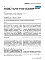
Figure 2 Overview of the TuMult algorithm. (a) Discretized copy number profiles of three t umors from t he same patient (yellow, ‘normal
copy number’; green, ‘loss’; red, ‘gain’). The eight breakpoints identified in the samples (dashed lines) divide the chromosome into seven
‘homogeneous segments’, A to G, in which copy number is constant in any sample. The profiles can be represented as amplitude vectors (see
Materials and methods), in which ‘up’ and ‘down’ breakpoints are distinguished by their position in the vector. A common breakpoint (gray
shading) appears as a non-zero value at the same position in the amplitude matrix. The frequency F
k
of each breakpoint is calculated from a
reference data set of independent samples. (b) An identical breakpoint score (IBS), characterizing the similarity of two profiles in terms of
chromosome breakpoints, is calculated for each pair of samples, and the pair displaying the highest level of similarity is selected. (c) The copy
number profile of the common precursor of the two samples is reconstructed based on their common breakpoints, represented by dashed lines
and black arrows. Edges are added between the common precursor (CP) and the two nodes, labeled with the aberrations defined by their
specific breakpoints, represented by gray arrows. Note that a breakpoint may be both common and specific, if its amplitude is larger in one of
the samples, like the ‘down’ breakpoint between segments A and B in this example. (d) Steps (b) and (c) are iterated until there is only one
node left in the front. (e) A ‘normal cell’ node has been added above the common ancestor of all tumors.
Letouzé et al. Genome Biology 2010, 11:R76
/>Page 4 of 19
the number of tumors involved, with a very small
increase in error rate for the copy number profiles of
the internal nodes.
The impact of noise and normal cell contamination
were evaluated on simulated trees with five leaves. The
results of TuMult and the parsimony method were unaf-
fected by noise with a standard devi ation below 0.10,

and normal cell contamination levels below 40%. The
performance of both algorithms then declined. The
decline was slightly faster for the TuMult algorithm,
which performed a little less well than the parsimony
method in terms of error rate at very high noise levels
(> 0.2; F igure 3b, middle panel) or at high levels of con-
tamination (> 60%; Figure 3b, bottom panel).
However, in the range of noise and contamination
expected for data of reasonably good quality, such as the
data analyzed below (noise < 0.11 and contamination
< 40%), the TuMult algorithm was much more efficient
than the parsimony method, giving the correct topology
in > 98% of cases, with an error rate in the internal node
profiles of < 1.6%.
Application to the study of bladder carcinogenesis
Five patients for whom two to four bladder cancer sam-
ples were avail able were analyzed with the TuMult algo-
rithm. In four cases, we had metachronous samples
obtained at different times during the course of the dis-
ease. In the remaining case (P3), we had samples from
different synchronous tumors removed from a cystect-
omyspecimen(Table1).Thetumorsfromthree
patients (P1 to P3) were analyzed with BAC arrays
(2,385 probes), and the tumo rs from two patients (P4
and P5) were analyzed with Illumina SNP arrays
(373,397 probes).
Figure 3 E valuation of the performance of TuMult and the parsimony method with simulated data. Simulated data were generated to
evaluate the performance of TuMult and the parsimony method for the reconstruction of tumor progression trees. The performance of each
algorithm was assessed under each set of conditions by generating 1,000 random trees and calculating (a) the percentage of the reconstructed
trees with the correct topology, and (b), for the trees with the correct topology, the percentage of probes with incorrect copy number status in

the internal nodes. Simulations were carried out for different numbers of tumors (upper panel), various levels of noise in the data (middle panel),
and various proportions of normal cells in the samples (bottom panel). The number of tumors analyzed (between 2 and 6), together with the
levels of noise (between 0.03 and 0.11) and contamination (10 to 40%) estimated for our experimental data are represented by yellow areas.
Letouzé et al. Genome Biology 2010, 11:R76
/>Page 5 of 19
The hypothesis of a monoclonal origin for all samples
was supported by the large number of shared chromo-
some aberrations (Figure 4) in all patients except P5. In
P5, we found that only a small proportion of the aberra-
tions present in tumor S5_C were common to S5_A and
S5_B, raising questions about whether tumor S5_C
resulted from the same initial c lone as S5_A and S5_B
but diverged early, or whether it had a different origin
but acquired a few similar events by chance.
Interestingly, sample S5_C was obtained from an inva-
sive tumor, whereas the other two samples from P5
were from superficial Ta tumors. Although S5_C was
detected less than 3 months after S5_B, our analysis
shows that these two samples displayed only a weak clo-
nal relations hip, if any. Note that our findings regarding
clonality are high ly consistent with clonality determina-
tions based on the partial identity score proposed by
Bollet et al. [18] (Additional file 1).
No linear evolution, in which one tumor could be
identified as the direct descendant of another tumor,
was observed . Instead, each tumor displayed a subset of
specific events occurring after the divergence of the
tumors. In some cases, the primary tumor may have
many more aberrations than the recurrence, as found
for S2_A and S2_B or S5_A and S5_B, consistent with

the finding of van T ilborg et al. [13] that tumor com-
plexity is not correlated with the chronological order in
which tumors are clinically detected. Thus, the aberra-
tions displayed by the primary tumor do not reliably
reflect the initial steps of tumor progression. By con-
trast, tumor progression trees make it possible to iden-
tify the events occurring at the start of tumorigenesis,
even from a set of very complex samples, as in patient
P3, in which a subset of ten early aberrations was identi-
fied, including two amplicons reported to be frequent in
bladder cancer [21-25], at 11q13.3 (Cyclin D1)and
8q22.2 (no known oncogene). The n umber of cancers
studied was too small for inference, with a satisfactory
level of statistical confidence, of the chronology of chro-
mosomal events in bladder cancer, but the most fre-
quently observed events on the initial edge of the tumor
progression trees were -9q (in four out of five tumor
progression trees), which is known to be one of the ear-
liest steps in most bladder cancers [26-28], and -11p (in
three out of five tumor progression trees). Finally, as the
aberrations observed on the same edge of a tumor pro-
gression tree presumably occurred during the same time
period, we investigated the co-occurrence of the most
frequent aberrations in b ladder cancer on the 21 edges
of our five tumor progression trees (see Materials and
methods). Despite the limited statistical power of our
test, due t o the small number of tr ees, -11p was shown
to occur on the same edge as -9q (P = 0.0025) and
–9p21.3 (CDKN2A tumor suppressor; P = 0.012) signifi-
cantly more frequently than would be expected by

chance. This suggests a possible synergic effect of these
three aberrations on tumor growth. Alternatively, the
co-occurrence of such events may have a mechanistic
cause, such as frequent chromosome rearrangement, as
between chromosomes 1 and 16 in Ewing sarcoma [29].
Application to the study of breast carcinogenesis
Fifteen of the 22 pairs of primary breast carcinomas and
ipsilateral recurrences studied by Bollet et al. [18] were
shown to have a monoclonal origin. We analyzed these
15 pairs with the TuMult algorithm. A linear evolution
was found in only one of the 15 pairs of tumors studied,
pair 14 (Figure 5a), all the other pairs displaying events
specific to the recurrence and events specific to the pri-
mary tumor (F igure 5b,c), consistent with the findings
of Kuukasjärvi et al. [30] regarding primary tumors and
metastases. A median of 17 aberrations occurred
between the normal cell and the common precursor, 14
aberrations occurred between the common precursor
and the primary tumor, and 26 aberrations occurred
between the common precursor and the ipsilateral
recurrence (Figure 5d). By contrast to what has been
observed for bladder cancer, the number of aberrations
specific to the recurrence was significantly higher than
the number of aberrations specific to the primary tumor
(P = 0.008). As all patients underwent radiotherapy and
Table 1 Clinical data for the 13 bladder samples analyzed
with the TuMult algorithm
Sample Patient Sex Stage Grade Surgery
time
Copy number

analysis
S1_A P1 M T2 G2 t0 BAC array-CGH
S1_B P1 M T1 G3 t0 + 21.8
months
BAC array-CGH
S2_A P2 M T3 G3 t0 BAC array-CGH
S2_B P2 M T3 G3 t0 + 2.1
months
BAC array-CGH
S3_A P3 M T4 G3 t0 + 157
months
BAC array-CGH
S3_B P3 M T4 G3 t0 + 157
months
BAC array-CGH
S3_C P3 M T4 G3 t0 + 157
months
BAC array-CGH
S3_D P3 M T4 G3 t0 + 157
months
BAC array-CGH
S4_A P4 F T1 G2 t0 SNP array
S4_B P4 F T1 G3 t0 + 14.4
months
SNP array
S5_A P5 M Ta G1 t0 SNP array
S5_B P5 M Ta G1 t0 + 7.8
months
SNP array
S5_C P5 M T3 G3 t0 + 10.3

months
SNP array
In the ‘ Surgery time’ column, t0 refers to the time of occurrence of the
primary tumor.
Letouzé et al. Genome Biology 2010, 11:R76
/>Page 6 of 19
some also underwent chemotherapy between the pri-
mary tumor and the recurrence, it is unknown whether
the higher complexity of the recurrences resulted from
treatment or were intrinsic to the tumor progression
process.
The 15 tumor progression trees were used to discrimi-
nate between early and late events in breast cancer
development. We conside red the 17 aberrations defined
as frequent in breast carcinoma by Hwang et al. [31],
determining the frequency of each of these aberrations
on each edge of the trees. We then used a two-tailed
Fisher’s exact test to determine whether each aberration
was associated with the early step (between the normal
cell and the common precursor) or the late step
(between the common precursor and the primary
tumor) of tumor progres sion. The edge between the
common precursor and the recurrence was not consid-
ered because some of the aberrations on this edge may
have resulted from radiotherapy. Five events were found
to be significantly associated with the early step: +1q,
-6q, -8p, +8q, and -16q (Table 2). Consiste nt with these
findings,+1q,-8p,+8q,and-16qwereshowntobe
among the most frequent aberrations (≥35%) in ductal
carcinoma in situ, a precursor of invasive breast carci-

noma [31]. The other two aberrations also shown to be
common in ductal carcinoma in situ by Hwang et al.,
Figure 4 Bladder tumor progression trees reconstructed with the Tu Mult algorithm. Thirteen samples from five patients were analyzed
with the TuMult algorithm to reconstruct the tumor lineage and sequence of chromosomal aberrations in each case. Aberrations are annotated
as follows: (–) homozygous deletions, (-) losses, (+) gains, (++) amplicons. Aberration boundaries are indicated in terms of chromosome
cytobands. Tumor progression trees with aberrations indicated in terms of homogeneous segments are available, together with the segment
description tables, from the TuMult web page [43]. Losses of chromosome arms 9q and 11p are underlined, along with homozygous deletions
of 9p21.3. The aberrations -9q and -11p were the most frequent early events in the tumor progression trees. In addition, -9q and -11p occurred
together on the same edge significantly more frequently than would be expected by chance (P = 0.0025). This was also true of -11p and
-9p21.3 (P = 0.012). Clinical details for each sample can be found in Table 1.
Letouzé et al. Genome Biology 2010, 11:R76
/>Page 7 of 19
-17p and +17q, were not identified as ‘early’ by our
approach. However, our findings do not conflict with
those of Hwang et al. for-17p,asthisaberrationwas
found in the common precursor in 40% of our trees, but
was not considered to be significantly early because it
also occurred in the late step in 20% of the trees. No
alteration was found to be significantly more frequent in
the late step, consistent with the conclusion of Hwang
et al. that ductal carcinoma in situ is a genetically
advanced lesion, with a degree of chromosome altera-
tion similar to that in invasive breast cancers.
Application to the study of metastatic progression in
prostate cancer
In a recent article, Liu et al. [19] analyzed anatomically
separate tumors from men who died from metastatic
prostate cancer. They showed that although individual
metastases displayed specific aberrations, all the samples
Figure 5 Accumulation of chromo some aberrations during breast cancer progression. Fifteen pairs of primary breast carcinomas and

ipsilateral recurrences were analyzed with the TuMult algorithm. Patients are denoted as in the original article by Bollet et al. [18]. (a) In patient
P14, all the aberrations of the primary tumor were found in the recurrence, consistent with a linear evolution. (b) In patient P13, both the
primary tumor and the recurrence display specific events, implying that the recurrence was not directly descended from the primary tumor. (c)
The proportion of all the aberrations in the tree occurring before the common precursor (white), between the common precursor and the
primary tumor (blue hatched) or between the common precursor and the recurrence (red hatched) is presented for each of the 15 patients. P14
is the only example of linear evolution among the 15 trees. (d) Boxplots of the number of aberrations occurring at each step in tumor
progression trees. CP, in the common precursor; PT, between the common precursor and the primary tumor; IR, between the common
precursor and the ipsilateral recurrence. **P-value < 0.01, as determined in a two-tailed paired t-test.
Letouzé et al. Genome Biology 2010, 11:R76
/>Page 8 of 19
from a given patient had a monoclonal origin, and
maintained a signature copy number pattern of the pre-
cursor metastatic cancer cell. The Affymetrix Genome-
Wide Human SNP Array 6.0 data from this article, com-
prising the copy number profiles of 58 metastatic sam-
ples taken from different anatomic sites in 14 patients,
areavailablefromtheGeneExpressionOmnibusdata-
base [32]. We used these data to reconstruct the tumor
progression tree in each patient with the TuMult algo-
rithm . Consistent with the conclusion of Liu et al., each
tree displayed a common precursor of all samples, with
a substantial number of aberrations (median = 26.5
events).
We first used the tumor progress ion trees to look for
recurrent events at the onset of metastasis. In each tree,
the common precursor of all metastases represents the
ancestral clone from which all the metastases spread,
and is thus likely to harbor the crucial alterations trig-
gering metastasis. We determined the frequencies of
gains and losses within the genome in the metastatic

precursor clones of the 14 tumor progression trees (Fig-
ure 6). Thirteen aberrations were detected in m ore than
half the precursors, including gains at 7p (57%), 8q
(86%), 10q21 (50%), 12q (57%) and Xp22 (50%), and
losses at 5q21 (50%), 6q14-21 (64%), 8p21 (93%), 13q13-
22 (71%), 16q22-24 (57%), 17p13-11 (79%), 21q22 (50%)
and 22q13 (50%). Loss of 8p21 (in 13 out of 14 cases)
andgainof8q24(in11outof14cases)werethemost
frequent events in our metastatic precursor clones, sug-
gesting that they may play a role in metastatic progres-
sion. Consistent with these observations are the findings
that gain of MYC (8q24) is associated with poor prog-
nosis in prostate cancer, and that the pattern of 8p21-22
loss with 8q24 gain is an independent risk factor for sys-
temic progression and cancer-specific death in this
disease [33].
For eight patients, the set of metastases included sev-
eral metastases from the same organ, either at the same
anatomic site (liver), or in the same type of organ, but
at different locations (lymph nodes and bone metas-
tases). We investigated whether metastases from a given
organ were more closely related to each other in the
trees than to metastases from other organs. The liver
metastases were systematically more closely related to
each other than to other metastases. They were always
derived from a single precursor (as in patient 21; Figure
7a), with specific events not found in the other metas-
tases (Figure 7b), forming a subtree in the tumor p ro-
gression tree. This finding is significant, since the
probability of observing such a pattern in the three

patients by chance, calculated as the proportion of all
the possible tree topologies in which liver metastases
form a subtree, is only P = 0.003. By contrast, lymph
node and bone metastases were often found together
with other metastases in the tumor progression trees
(Additional file 2). One possible interpretation of the
late divergence of liver metastases is that specific altera-
tions are required for liver invasion. Thus, all liver
metastases would be likely to arise from a subclone of
theprostatetumorwiththerequiredalterations.Alter-
natively, the invasion of the liver by one clone may be
the limiting step for metastatic spread in this organ,
Table 2 Early or late occurrence of the most frequent aberrations in breast carcinoma
Aberration Occurrence in the common precursor
(CP)
Occurrence between the CP and the primary
tumor
Association with early/late
events
+1q 53% 13% 0.050
a
-3p 7% 13% 1
-6q 40% 0% 0.017
a
-8p 60% 0% 0.00070
c
+8p 0% 7% 1
+8q 53% 0% 0.0022
b
-9p 27% 0% 0.10

-11q 20% 7% 0.60
+11q 0% 7% 1
-14q 27% 7% 0.33
+16p 0% 7% 1
-16q 47% 7% 0.035
a
-17p 40% 20% 0.43
+17q 20% 13% 1
-18p 7% 7% 1
-18q 27% 7% 0.33
+20q 0% 0% 1
a
P ≤ 0.05;
b
P < 0.01;
c
P < 0.001; Fisher’s exact test.
Letouzé et al. Genome Biology 2010, 11:R76
/>Page 9 of 19
with all the metastases in the liver resulting from the
dissemination of a single clone successfully colonizing
the organ. We favor this hypothesis because the alterna-
tive explanation would probably result in lymph node
and bone metastases being closely related too, and
because no organ-specific alterations were identified by
Liu et al.
Discussion
In this paper, we introduce a new method for unraveling
the succession of chromosome aberrations occurring
during the process of carcinogenesis. It has recently

been shown that copy number data for several samples
from the same patient can be used to demonstrate clon-
ality [18], or to elucidate the biology underlying relapse
[34] or metastasis [19]. However, a co mputational
approach for automatically reconstructing tumor
lineages and the sequence of chromosomal events from
high-definition copy number data was lacking. Several
algorithms for reconstructing trees from discrete charac-
ter vectors o r distance matrices have been developed in
phylogenetics [20,35-39], but particular features speci fic
to copy number data, in particular the cumulative nat-
ure of aberrations, made it necessary to develop a dedi-
cated algorithm.
OneofthekeyfeaturesoftheTuMultalgorithmis
that it focuses on chromosome breakpoints, rather than
aberrations, making it possible to reconstruct the ances-
tral chromosomal events from profiles with several
imbricated aberrations. As a result, the performance of
TuMult is little affected by the complexity of the trees,
unlike the parsimony method, the performance of which
declines rapidly with the occurrence of overlapping
aberrations. However, reasoning in terms of break points
introduces additional dif ficulties. First, an odd number
of common breakpoints may be identified for a given
chromosome. This occurs in the rare cases in which a
common breakpoint is erased by a subsequent break-
point of the opposite sign at the same location, or when
two independent aberrations share a common break-
point by chance. In this case, some of the information
required for inference of the s equence of events with

certainty is lacking, so TuMult reconstructs the scenario
involving the smallest number of changes. These rare
situations occur mostly in conditions in which a large
number of events have accumu lat ed, accounting for the
slight increase in error rates with in creasing numbers of
tumors. Second, the copy number profiles must be of
sufficiently high quality for the identification of common
breakpoints. With increasing noise and normal cell con-
tamination, the breakpoints may be shifted a few probes
away by segmentation algorithms. A tolerance threshold
was introduced to deal with such samples. However, as
increasing this threshold decreases the specificity of
common breakpoints, we recommend the discarding of
samples of very low quality (noise standard deviation >
0.12 or normal cell contamination > 50%) when analyz-
ing data with TuMult. If these precautions are taken,
the tumor progression trees reconstructed with TuMult
are highly reliable, as demonstrated from our analysis of
simulated data.
The applications of TuMult in cancer research are
numerous. First, TuMult makes it possible to go back in
time, reconstructing the genomic profiles of ancestral
tumor clones of p articular interest that are not accessi-
ble by sampling. We have shown that, in both bladder
and breast cancers, recurrences do not generally arise
directly from the primary tumor. The primary tumor
thus displays many specific events and is poorly repre-
sentative of the initial tumor progression step. By
Figure 6 Frequency of gains and losses in the metastatic precursor clones of 14 patients with metastatic prostate cancer. Fourteen
patients with various metastatic samples taken from different anatomic sites were analyzed with the TuMult algorithm to generate the lineage

of the metastases and to reconstruct the copy number profile of the common precursor of all metastases in each patient. The frequency of
gains (in red) and losses (in green) in the genome were calculated for these 14 metastatic precursor clones.
Letouzé et al. Genome Biology 2010, 11:R76
/>Page 10 of 19
contrast, the common precursor of all samples usually
displays a small set of aberrations, even if all the tumors
studied have complex profiles. This strategy may be of
particular interest when trying to identify the initial
events in carcinogenesis, particularly for cancers in
which early lesions are rarely accessibl e. Another ances-
tral clone of particular interest was highlighted when
studying the metastatic process in prostate cancer. We
were able to reconstruct the copy number alterations of
the metastatic precursor clone giving rise to all the
metastases in each patient. A few recurrent aberrations
were identified in these clones. These aberrations poten-
tially play an important role in metastatic spread and
may be good predictors of metastasis in prostate cancer.
Second, tumor progression trees could be used i n
integrative studies aiming to develop a general model of
Figure 7 Metastases spreading in a patient with prostate cancer. Five metastases were removed from patient 21 (data from Liu et al. [19]),
including three liver metastases (21-2a, 21-2b and 21-2c), one adrenal metastasis (21-3) and one bone metastasis (21-6). (a) Tumor progression
tree reconstructed with the TuMult algorithm. The three liver metastases have a longer clonal relationship than the other metastases, all being
derived from common precursor 3. (b) Copy number profiles of chromosome 2 in the five metastases. Four common aberrations, delimited by
dashed lines, occurred in the common precursor of all the samples. The seven circled aberrations are specific to the three liver metastases,
showing these tumors diverged later in the tumor progression tree. These aberrations appeared in common precursor 3, from which the liver
metastases are derived.
Letouzé et al. Genome Biology 2010, 11:R76
/>Page 11 of 19
tumor progression. In such studies, individual tumor

progression trees are much more informative than a col-
lection of individual samples, as the relative times at
which aberrations occurred is already known in each
patient. As a proof-of-concept, with only 15 breast
tumor progression trees, we were able to identify most
of the early aberrations previously described as c harac-
teristic of ductal breast carcinoma in situ, the precursor
lesion of invasive breast cancers [31,40], despite our
data corresponding only to invasive samples. Conversely,
the analysis of cases with both superficial and invasive
tumors may facilitate identification of the genes respon-
sible for invasiveness, through studies of the aberrations
occurring between the common precursors and invasive
samples.
Finally, the tumor lineage per se may provide insight
into the spread of cancerous cells to different parts of
the organ, or di fferent parts of the body. Analysis of the
copy number profiles of metastases in the data set from
the study by Liu et al. [19] revealed the relationships
between the metastases in the different organs, showi ng
that liver metastases always diverged from a single pre-
cursor clone.
One factor limiting the application of TuMult is the
need to have access to several tumors from the same
patient, either at different time points during the disease
(recurrences), or from different sites at a single time
point. Most tumors are thought to be hete rogeneous,
consisting of a mixture of clones that have diverged
from the same initial cancer cell. The microdissection of
distantpartsofasingletumormaythereforemakeit

possible to reconstruct thesequenceofaberrations
occurring during the clonal development of the tumor,
providing access to early and late events, just like the
analysis of samples from different tumors [41]. Using
ultra-deep sequencing, Campbell et al. [42] were able to
infer the interrelationshipsbetweensubclonesintwo
tumors. Most genomic analyses to date have focused on
the search for similarities in large tumor data sets, with
the aim of identifying the fundamental mechanisms of
cancer. The next step may be to dig deeper into the
dynamic pathways of cancer progression by analyzing
the unique succession of changes driving carcinogenesis
in each patient.
Conclusions
We report here a novel computational approach for
unraveling the successive copy number alterations driv-
ing carcinogenesis. We have shown that TuMult is
highly reliable for reconstructing both tumor lineage
and the copy number profiles of ancestral tumor cl ones,
significantly outperforming the parsimony method.
TuMult is a new tool of great interest for researchers
seeking to develop a profound understanding of the
development of cancer from the analysis of several sam-
ples. The annotated R code of the program is provided,
together with detailed user instructions and examples of
formatted data [43].
Materials and methods
Patients and bladder tumor samples
We obtained 28 bladder tumor samples from patients
admitted between 1993 and 2002 to the Henri Mondor

Hospital. Thirteen of these samples were multiple
tumors from five patients (two to four metachronous or
synchronous samples per patient; Table 1). The other 15
samples came from 15 independent patients (Additional
file 3) and were used as the reference data set for esti-
mation of the frequency of breakpoints at each location
in the bladder SNP data. All subjects provided informed
consent and the study was approved by the ethics com-
mittee of Henri Mondor Hospital. Flash-frozen tissue
samples were stored at -80°C immed iately after transur-
ethral resection or cystectomy. DNA was extracted with
the cesium chloride [44] or proteinase K/phenol/chloro-
form method. DNA pur ity was assessed by determining
the ratio of absorbances at 260 and 280 nm. DNA con-
centration was determined with a Hoechst dye-based
fluorescence assay [45].
BAC array CGH
Eight bladder tumors from three patients were analyzed
with HumArray 2.0 arrays, consisting of 2,385 BAC
clones covering the human gen ome with an average
resolution of 1.3 Mb, as previously described [46]. These
arrays were obtained from the UCSF Cancer Center
Array CGH Core Facility. Probes were labeled and
hybridization was carried out as described elsewhere
[47]. Images were analyzed with SPOT 2.0 software [48].
Poor-quality spots were removed in a pre-processing
step: only spots with a reference signal intensity above
25% of the background reference signal (the 4,6-diami-
dino-2-phenylindole (DAPI) signal) were considered reli-
able. Spots located in zones of spatial bias were ignored

[49]. No value was assigned to 25 BACs in the data, and
these BACs were therefore eliminat ed from the analysis.
Each BAC was assigned ‘gain’, ‘normal’ or ‘loss’ status,
using the GLAD segmentation algorithm [50]. BACs
with log2 ratios below -0.8 and over 0.8 were assigned
‘homozygous deletion’ and ‘amplificat ion’ status,
respectively.
SNP arrays
We analyzed 20 bladder tumors, comprising 15 indepen-
dent tumors and 5 multiple tumors from two patients,
with Illumina HumanCNV370 Genotyping BeadChips
(Illumina Inc.). Hybridization was performed by Integra-
Gen (Evry, France), according to the instructions
Letouzé et al. Genome Biology 2010, 11:R76
/>Page 12 of 19
provided by the array manufacturer. Fluorescent signals
were imported into BeadStudio software (Illumina Inc.)
and normalized. The normalized fluorescence signals for
a sample were c ompared with the signal intensities of a
set of reference genotypes in Beadstudio software, and
the log2 ratios between the sample and reference signals
(log R ratios (LRR)) were calculated as previously
described [51]. In addition, the B-allele frequency (BAF)
for the sample was estimated, based on the reference
genotype clusters [51]. Segmentation was carried out
with the BAFsegmentation algorithm [52,53], with
amplitude (ai.thr) and size (ai.size) thresholds for signifi-
cant allelic imbalance detection set at 0.53 and 10,
respectively. As this method requires heterozygous
SNPs, the × and Y chromosomes of the m ale patient

were segmented based on LRR, using the CBS algorithm
[54] (R package DNAcopy [55]) with default settings
except for the significant level for accepting change-
points (a), which was set to 0.001, and a size threshold
of 10 SNPs for signifi cant aberrations , which was added
to ensure concordance with the smoothing for other
chromosomes. A discrete copy number status w as then
assigned to each segment, based on its median LRR
value. The zero level for normal copy number segments
was first determined as the median LRR in regions of
allelic balance, as previously decribed [56]. Segments
with a median LRR more than 0.05 above the zero level
were assigned ‘gain’ status and segments with a median
LRR more than 0.5 above the zero level were assigned
‘amplified’ status. Segments with a median LRR more
than 0.05 below the zero level were assigned ‘loss’ status
and segments with a median LRR more than 0.5 below
the zero level were assigned ‘homozygous deletion’ sta-
tus. SNP data for breast samples were kindly provided
by Bollet et al., and the details of array processing and
copy number alteration determination for these samples
are provided in the corresponding article [18].
Generation of tumor lineage trees
Overview of the method
The clonal development of several tumors in a patient
can be represented as a ro oted tree, where the root
represents the normal cell (NC), the leaves are the
tumors removed from the patient, and the intermediate
nodes are the common precursors of the observed sam-
ples. We want to reconstruct the most likely tumor line-

age and to infer, simultaneously, the copy number
profiles of the intermediate nodes. In other words, we
want to reconstruct the copy number profiles of the
common ancestors of the tumors. We use a botto m-up
agglomerative strategy to do this. Let the Front be the
set of nodes with no upstream edge at a given step of
tree reconstruction. Initially, the Front is the set of
tumors removed from the patient. At each step of the
algorithm, the two closest nodes in the Front,interms
of breakpoints, are joined. The copy number profile of
their common precursor is inferred, and the common
precursor replaces the two nodes in the Front. This step
is iterated until the Front contains only one node: the
common ancestor of all samples.
Definition of breakpoint and amplitude vectors
We define a chromosome breakpoint as a change in
copy number status between two consecutive probes.
Chromosome breakpoints are also defined at chromo-
some ends, where copy number differs from the normal
value. Before tumor lineage reconstruction, each chro-
mosome is divided into ‘homogeneous segments’ delim-
ited by all the brea kpoints identified in the samples
from the patient. A segment is thus a continuous set of
probes for which copy number is constant in any sample
from the patient. Let N be the number of segments
delimited on the chromosome. For each sample, the
copy number profile on the chromosome can be repre-
sented as a vector s ε {-2,-1,0,1,2}
N
where s

j
repre-
sents the copy number of segment j (-2, homozygous
deletion; -1, l oss; 0, normal; 1, gain; 2, amplification). A
breakpoint vector b is defined from s as follows:
bs
bss iN
bs
iii
NN
11
1
1
2
=
=− ≤≤
=−
−
+
,
There is there fore a breakpoint between segments i -
1andi if, and only if, b
i
≠ 0. Each breakpoint is charac-
terized by its sign: ‘up’ if b
i
>0,‘down’ if b
i
<0,andits
amplitude |b

i
|.
We need to consider ‘up’ and ‘down’ breakpoints sepa-
rately. We have therefore simplified the notation, defin-
ing breakpoint amplitude vector a as follows:
ab ifb
abifb
ii i
Ni i i
=≥
=− ≤
++
0
0
1
The amplitude vectors of all c hromosomes are then
joined end-to-end to form the amplitude vector of the
whole profile. In the following, a refers to the amplitude
vector of the whole profile of the tumor. The generation
of the segment, breakpoint and amplitude vectors is illu-
strated in Additional file 4.
Note that the functions associating a se gment vector s
with a breakpoint vector b and a breakpoint vector b
with an amplitude vector a are bijections. In other
words,anyamplitudevectorcorrespondstoaunique
breakpoint vector and a unique segment vector.
Biological viability of a chromosome breakpoint vector
All aberrations involve the occurrence of two break-
points (one ‘up’ and o ne ‘down’), so a breakpoint vector
b represents a biologically viable chromosome only if

Letouzé et al. Genome Biology 2010, 11:R76
/>Page 13 of 19
‘up’ and ‘down’ breakpoints are balanced:
b
i
i
N
=
+
∑
=
1
1
0
This condition is verified by definition in the tumor
breakpoint vectors, but it must be checked for each
chromosome when reconstructing the copy number
profiles of common precursors.
Definition of a common breakpoint
We define a common breakpoint of tumors T
i
(repre-
sented by its breakpoint amplitude vector a
i
)andT
j
(represented by vector a
j
)asabreakpointofthesame
sign observed at the same location in the two samples,

that is, belonging to
ka a
k
i
k
j
/,>>
{}
00
. An adjustable
tolerance threshold was introduced to recognize as com-
mon breakpoints, breakpoints located very close
together, for which the slight differen ce in location
probably resulted from sm all discrepancie s in the
smoothing process. For bladder samples, the 95th per-
centiles of the errors in the location of the breakpoints,
estimated by permuting the markers within each seg-
ment and re-segmenting 100 times, were used as toler-
ance thresholds. The Bollet and Liu data were already
discret ized. We therefore used a threshold of ten probes
for these data sets, consistent with the thresholds esti-
mated for our bladder samples analyzed with SNP
arrays.
Identical breakpoint score
At each step of the algorithm, the two nodes that sepa-
rated most recently in the tumor line age are joined. As
chromosome aberrations accumulate during tumor
development and are passed on to daughter cells, we
can assume that the later two tumor clones separate,
the more chromosome breakpoints they will have in

common. We defined an identical breakpoint score
(IBS) to quantify the number of breakpoints common to
two nodes.
Let us consider two nodes, N
i
and N
j
, characterized by
their amplitude vectors, a
i
and a
j
. We first define the
common amplitude vector a
ij
as the amplitude vector of
breakpoints common to nodes N
i
and N
j
:
aaa
k
ij
k
i
k
j
=
()

min ,
As very frequent breakpoints are more likely than rare
breakpoints to occur independently, by chance , on sev-
eral occasions, the added value of each breakpoint is
weighted down according to its frequency F
k
in a refer-
ence data set of independent tumors, as proposed by
Bollet et al. [18]. Three data sets were used to estimate
the frequencies of ‘up’ and ‘down’ breakpoints at each
location: 50 previously published bladder tumors for
BAC arrays [46], a set of 15 independent bladder tumors
for SNP arrays, and the s ame set of 44 control samples
used by Bollet et al. for breast tumors.
The IBS is simply the number of breakpoints common
to the two nodes, weighted by their frequency in the
reference data set:
IBS a a a F
ij
k
ij
k
k
,
()
=−
()
∑
1
Similarly, we define the distance between two nodes as

the number of breakpoints differing between the two
profiles, weighted by their frequency in the reference
data set:
Daa a a F
ij
k
i
k
j
k
k
,
()
=−−
()
∑
1
At each step of the algorithm, the two nodes from the
Front with the highest IBS are joined. If several pairs
have the same IBS, the pair with the smallest distance is
chosen.
Generation of the copy number profile of the common
precursor of two samples
At each step of the algorithm, the profile of the com-
mon precursor of the two no des joined, CP(a
i
,a
j
), is
inferred. This profile is reconstructed chromosome by

chromosome, through the identificatio n of breakpoints
common to the two nodes. In this paragraph, notations
a and b therefore refer to the amplitude and breakpoint
vectors of a single chromosome.
First, the common breakpoints are identified by com-
puting the common amplitude vecto r of the two nodes,
a
ij
, as described above:
aaa
k
ij
k
i
k
j
=
()
min ,
The balance between the ‘up’ and ‘down’ breakpoints
in this vector is then checked, because an unbalanced
profile (for example, one common breakpoint ‘up ’ and
no common breakpoint ‘down’)doesnotdefineaviable
copy number profile. This is done by inferri ng the com-
mon breakpoint vector b
ij
corresponding to a
ij
,and
checking the balance between ‘up’ and ‘down’ break-

points by calculating the sum δ of all the breakpoints
affecting the chromosome:

=
∑
b
k
ij
k
Two situations emerge at this point. First, if δ =0,‘up’
and ‘down’ breakpoints are balanced, the amplitude
Letouzé et al. Genome Biology 2010, 11:R76
/>Page 14 of 19
vector of the common precursor is given directly by:
CP a a a
ij ij
,
()
=
Second, if δ ≠ 0, ‘up’ and ‘down’ breakpoints are unba-
lanced. The set of breakpoints in the common precursor
doesnotdefineaviablecopynumberprofileand
requires correction (see next section) to restore the
equilibrium.
Correction of unbalanced chromosomes
In rare cases, the number of common breakpoints of each
sign (’up’ and ‘down’) differ for a given chromosome:

=≠
∑

b
k
ij
k
0
There are two possible reasons for this (Additional file
5). In the first case, if several aberrations appearing
independently in several lineages have, by chance, a
breakpoint in common, this breakpoint will be consid-
ered as a common breakpoint and incorporated into the
common precursor without a counterpart of the oppo-
site sign, leading to an unbalanced profile. In this case,
the actual profile of the common precursor is obtained
by removing the f alse common breakpoint. In the sec-
ond case, if two aberrations successively affect two
neighboring segments, a breakpoint may be erased by
the occurrence of a breakpoint of the opposite sign at
the same location. One of the breakpoints defining a
common aberration may therefore be missing in one of
the two descendant nodes, leading to an unbalanced
profile. In this case, the actual profile of the common
precur sor is obtained by adding the breakpoint that has
been erased to the profile of the common precursor.
Thus, to restore breakpoint equilibrium in the com-
mon precursor, we need to either remove a breakpoint
of sign(δ) from the common breakpoint vect or (the first
case), or add a breakpoint of sign(-δ)chosenfromthe
breakpoints specific to one of the two samples (the sec-
ond case). As each choice generates a different common
precursor and a different sequence of events for the

chromosome considered, each possible modification is
automatically evaluated in terms of the sequence of
events it would generate. The breakpoint correction that
does not lead to an impossible event (such as a segment
deviating from the set of authorized values {-2, -1, 0, 1,
2}) and minimizes breakpoint usage is selected (Addi-
tional file 6), and the status of the breakpoint is cor-
rected in the profile of the common precursor.
The particular case of amplicons
Amplicons are known to originate from mechanisms
different from those responsible for generating losses
and gains, including unscheduled DNA replication or
inverted duplicatio ns [57]. In particular, amplicons can-
not be consid ered as an accumulation of gains target ing
the same region. We therefore treated amplicons sepa-
rately from other aberrations. Once the copy number
profile of the common precursor has been recon-
structed, amplicons common to both descending nodes
are incorporated into it, and amplicons specific to one
of the descendant nodes are placed on the relevant edge.
Visualization of the trees
The tumor progression trees produced by the TuMult
algorithm were exported in .dot format. Images were
produced from the .dot files with the open source graph
visualization software Graphviz [58].
Analysis of simulated tumor progression trees
Simulation of tumor progression trees
We implemented an algorithm to generate simulated
tumor progression trees to validate the reconstruction
methods. First, a common precursor is created from the

‘Normal tissue’ node. Then, at each step of the algo-
rithm, a node is randomly chosen in the front, from
which two new nodes are created, until the required
number of tumors is obtained. The profile of each new
node is determined as follows: 1, random selection of
the number n
ab
of aberrations to add, between 3 and 15
(in line with the numbers observed in experimental
trees); 2, random selection of n
ab
pairs of ‘up’ and
‘down’ breakpoints; 3, calculation of the copy number
profile obtained by adding the aberrations thus d efined
to the previous node. Aberrations that would lead to an
impossible copy number (out of {-2, -1, 0, 1 2}) are dis-
carded and replaced by a new randomly generated aber-
ration to avoid the creation of meaningless profiles. This
algorithm was used to simulate tumor progression trees
of random topologies, with various numbers of tumors.
We obtained realistic copy number profiles by setting
the number of probes to 2,360, as in our reference CGH
data set for bladder tumors, and weighting the random
sampling of breakpoints according to their frequency in
this reference data set.
Effects of noise and normal cell contamination
We investigated the impact of noise in the log ratio and
normal cell contamination on the performance of the
method by generating simulated log ratio signals from
the discrete copy number profiles of each node. For

each copy number st atus N, the theoretical log ratio
value was calculated as a function of the percentage C
of normal cells in the sample:
log logratio
NCC
=
×−
()
+×
⎛
⎝
⎜
⎜
⎞
⎠
⎟
⎟
12
2
Letouzé et al. Genome Biology 2010, 11:R76
/>Page 15 of 19
Noise was then simulated by adding random values
drawn from a normal distribution with a m ean of 0 and
a standard deviation of S. Simulations were carried out
for values of C from 0 to 0.8 (80% of normal cells in the
sample), and values of S from 0 to 0.2. The values of S
in our experimental data, estimated as the standard
deviation of the difference between raw and smoothed
log ratios after segmentation, were between 0.03 and
0.11. The percentage C of normal cells in each sample

was between 10 and 40%, as assessed by hematoxylin
and eosin staining of the histological sections adjacent
to those analyzed.
Reconstructing tumor progression trees with the parsimony
method
The parsimony method [39] identifies the tree with the
minimum number of changes from a set of leaves char-
acterized by discrete character vectors. It could therefore
be used to benchmark the TuMult algorithm. For this
purpose, each tumor profile was divided into N ’homo-
geneous segments’, as in the preliminary step for the
TuMult algorithm, and represented as a vector s ε {-2,
-1,0,1,2}
N
where s
j
is the copy number of segment j.
These discrete vectors were used as an input for the
pars program of the Phylip package [20].
Evaluation of the reconstructed tree
We evaluated the two methods by comparing each
reconstructed tree with the original simulated tree. We
first checked that the topology of the reconstructed tree,
and hence the inferred tumor lineage, was identical to
that in the simulated tree. W e did this by calculating
the Robinson-Foulds distance [59] between the two
trees with the treedist program in the Phylip package
[20]. A distance of zero indicates that the trees are iden-
tical. For each simulation data set, we calculated the
percentage of the trees correctly inferred by each algo-

rithm (Robinson-Foulds distance = 0). Then, for the
trees with the correct topology, we checked that the
copy number profiles of the internal nodes (correspond-
ing to ancestral clones) were correctly reconstructed.
We did this by calculating, for each reconstructed tree,
the proportion of probes per node with a discrete copy
number status different from that in the original simu-
lated tree.
Determination of co-occurring events in bladder
carcinogenesis
If two aberrations a re found on the same edge of a
tumor progression tree, they must have occurred in the
same time interval. Therefore, if two aberrations have a
strong synergistic effect on tumor growth, they would
be expected to be found on the same edge of a tumor
progression tree significantly mor e frequently than
wouldbeexpectedbychance.Wedefinedasetof
aberrations frequently observed in bladder cancer on the
basis of their frequency in the reference data set of 50
samples. Gains and losses were considered to be fre-
quent in bladder cancer if they occurred in more than
20% of samples, whereas amplicons and homozygous
deletions were considered frequent if they occurred in
more than 10% of samples. Only aberrations found in at
least three edges in the tumor progression trees were
retained for further analysis. The co-occurrence of each
pair of aberrations was then assessed by Fisher’sexact
tests, with correction for multiple testing, as previously
described [60], using the q-value package in the R com-
puting environment. The false discovery rate was set at

15%.
Identification of early and late events in breast
carcinogenesis through the integration of individual
tumor progression trees
The tumor progression trees obtained from 15 pairs of
primary breast carcinomas and ipsilateral recurrences
were used to discriminat e between early and late events
in this disease. These trees contain three edges: one
edge from the normal cell to the common precusor
(CP), one edge from the CP to the primary tumor, and
one edge from the CP to the recurrence. We therefore
defined an aberration as early if it occurred between the
normal cell and the CP, and as late if it occurred
between the CP and the primary tumor. Aberrations
occurring between the CP and the recurrence were not
considered because they may have resulted from radio-
therapy administered between the primary tumor and
the recurrence. The 17 chromosomal aberratio ns identi-
fied as common in breast carcinoma by Hwang et al.
[31] were analyzed . We first calculated the frequency of
each aberration as an early or late step in the 15 tumor
progression trees. As these aberrations span whole chro-
mosome arms, w e considered an aberration to be pre-
sent on an edge if 60% of the probes on t his arm were
aberrant. Finally, we used two-tailed F isher’s exact tests
to determine whether each aberration was significantly
more present in the early or late step of carcinogenesis.
Availability
The TuMult algorithm was implemented in the R lan-
guage. The annotated code is provided, together with

detailed instructions for use and examples of formatted
data [43]. CGH and SNP data for the 78 bladder tumors
used in this study (CGH data comprises 8 multiple
tumors and t he reference data set of 50 samples; SNP
data comprises 5 multiple tumors and the reference
data set of 15 samples) are available through Gene
Expression Omnibus [32] accession number [GEO:
GSE19195].
Letouzé et al. Genome Biology 2010, 11:R76
/>Page 16 of 19
Additional material
Additional file 1: Consistency of tumor progression trees and the
partial identity score for sample clonality. The partial identity score
was developed by Bollet et al. [18] to determine whether two samples
have a monoclonal origin. We investigated the consistency of our results
with this approach by investigating the clonality of our bladder samples
with the partial identity score (top), and reconstructing tumor
progression trees for the pairs of breast samples characterized as non-
clonal in the paper by Bollet et al. (bottom). (a) The partial identity
scores were calculated for each pair of bladder tumors analyzed. The
distributions of these scores for pairs of samples from different patients
were calculated from the reference data sets (left, BAC array data; right,
SNP data). The 95% quantile, used by Bollet et al. as the threshold for
classifying a pair as monoclonal, is indicated as a red line. The only pairs
of samples from the same patient with a partial identity score below the
threshold were those involving sample S5C. Detailed numbering of pairs
for CGH data: 1, S1A-S1B; 2, S2A-S2B; 3, S3A-S3D; 4, S3B-S3D; 5, S3C-S3D;
6, S3A-S3B; 7, S3A-S3C; 8, S3B-S3C. Detailed numbering of pairs for SNP
data: 1, S4A-S4B; 2, S5A-S5B; 3, S5A-S5C; 4, S5B-S5C. (b) The tumor
progression tree obtained for the pair of breast tumors P2, classified as

non-clonal by Bollet et al. TuMult identified no common events between
the samples. (c) Boxplots of the number of aberrations occurring at each
step in the tumor progression trees obtained for true recurrences (left) or
new primary tumors (right). CP, in the common precursor; PT, between
the common precursor and the primary tumor; IR, between the common
precursor and the ipsilateral recurrence. Very few events are found in the
common precursors of the trees for new primary tumors, consistent with
their low partial identity scores.
Additional file 2: Tumor progression trees of metastatic prostate
cancers with several metastases from the same anatomic site or
type of organ. (a) Tumor progression trees of three patie nts with
several metastases from the same anatomic site (liver). Liver samples
were always more closely related to each other than to metastases from
the other organs. In each tree, the liver samples are derived from a
single common precursor, with a substantial number of events not
encountered in the other samples. (b) Tumor progression trees of six
patients with several metastases from the same type of organ but at
different anatomic sites (lymph node and/or bone metastases). The
tumors from the same type of organ are associated in P24, P28 and P30,
but not in P17, P32 and P33.
Additional file 3: Clinical data for the 15 bladder samples
constituting the reference data set for bladder SNP data.
Additional file 4: Segmentation of the profiles and generation of
the amplitude vectors. Generation of the amplitude matrix. (a)
Discretized copy number profiles of three tumors for a given
chromosome (yellow, ‘normal copy number’; green, ‘loss’; red, ‘gain’). The
four breakpoints identified in the samples (dashed lines) divide the
chromosome into five ‘homogeneous segments’. (b) The profiles are
equally well represented in a segment matrix, in which the copy number
for each segment and each sample is encoded by an integer (-1, loss; 0,

normal; 1, gain), in a breakpoint matrix, in which each value represents
the difference in copy number between two adjacent segments, or an
amplitude matrix, in which ‘up’ and ‘down ’ breakpoints are distinguished
by their position in the vector. A common breakpoint (gray regions)
appears as a number of the same sign at the same position in the
breakpoint matrix, or as a non-zero number at the same position in the
amplitude matrix.
Additional file 5: Two scenarios lead to an unbalanced chromosome
in the common precursor. (a) Left: the two tumors independently
acquire two different aberrations with a breakpoint in common. Right:
the ‘up’ breakpoint between segments B and C in the common
precursor is lost in tumor 2 due to the loss of the neighboring segment
C. (b) In both cases, only one breakpoint remains common to both
samples, resulting in an unbalanced chromosome for their common
precursor.
Additional file 6: Correction of an unbalanced chromosome. Detailed
procedure of the correction of chromosomes with unbalanced ‘
up’ and
‘down’ breakpoints.
Abbreviations
BAC: bacterial artificial chromosome; CGH: comparative genomic
hybridization; CP: common precursor; IBS: identical breakpoint score; SNP:
single nucleotide polymorphism.
Acknowledgements
We thank Nicolas Servant for providing the discretized copy number profiles
of breast tumor samples, Tatiana Popova for assistance in the analysis of
bladder SNP data, and Alain Aurias for his useful advice. This work was
supported by the Centre National de la Recherche Scientifique, the Institut
National de la Santé et de la Recherche Médicale, the Institut Curie, the
Institut National Contre le Cancer, the Ligue Nationale Contre le Cancer (EL,

FR, accredited team), the Cancéropôle Ile de France and the Groupement
d’Entreprises Françaises dans la Lutte contre le Cancer. Eric Letouzé was
supported by a fellowship from the French Ministry of Education and
Research and the Association pour la Recherche sur le Cancer.
Author details
1
INSERM, UMR-S 973, MTi, Université Paris Diderot - Paris 7, 35 rue Hélène
Brion, 75205 Paris Cedex 13, France.
2
Institut Curie, Centre de Recherche,
Paris, F-75248 France.
3
CNRS, UMR 144, 26 rue d’Ulm, 75248 Paris Cedex 05,
France.
4
INSERM, Unité 955, Créteil F-94000, France.
5
AP-HP, Groupe
Hospitalier Albert Chenevier - Henri Mondor, Département de Pathologie,
Créteil F-94000, France.
6
Département d’Oncologie Radiothérapie, Institut
Curie, 26 rue d’Ulm, 75248 Paris Cedex 05, France.
Authors’ contributions
EL, FR, FG and YA came up with the idea for this study. EL developed and
implemented the method under the supervision of FG. YA provided bladder
samples and clinical information. MB provided breast cancer data. All
authors participated in the evaluation of the results. EL wrote the
manuscript under the supervision of FG and FR. All of the authors have read
and approved the final manuscript.

Received: 12 April 2010 Revised: 25 June 2010 Accepted: 22 July 2010
Published: 22 July 2010
References
1. Hanahan D, Weinberg RA: The hallmarks of cancer. Cell 2000, 100:57-70.
2. Nowell PC: The clonal evolution of tumor cell populations. Science 1976,
194:23-28.
3. Vogelstein B, Fearon ER, Hamilton SR, Kern SE, Preisinger AC, Leppert M,
Nakamura Y, White R, Smits AM, Bos JL: Genetic alterations during
colorectal-tumor development. N Engl J Med 1988, 319:525-532.
4. Fearon ER, Vogelstein B: A genetic model for colorectal tumorigenesis.
Cell 1990, 61:759-767.
5. Desper R, Jiang F, Kallioniemi OP, Moch H, Papadimitriou CH, Schaffer AA:
Inferring tree models for oncogenesis from comparative genome
hybridization data. J Comput Biol 1999, 6:37-51.
6. Desper R, Jiang F, Kallioniemi OP, Moch H, Papadimitriou CH, Schaffer AA:
Distance-based reconstruction of tree models for oncogenesis. J Comput
Biol 2000, 7:789-803.
7. Hoglund M, Gisselsson D, Mandahl N, Johansson B, Mertens F, Mitelman F,
Sall T: Multivariate analyses of genomic imbalances in solid tumors
reveal distinct and converging pathways of karyotypic evolution. Genes
Chromosomes Cancer 2001, 31:156-171.
8. Bulashevska S, Szakacs O, Brors B, Eils R, Kovacs G: Pathways of urothelial
cancer progression suggested by Bayesian network analysis of
allelotyping data. Int J Cancer 2004, 110:850-856.
9. Beerenwinkel N, Rahnenfuhrer J, Kaiser R, Hoffmann D, Selbig J, Lengauer T:
Mtreemix: a software package for learning and using mixture models of
mutagenetic trees. Bioinformatics 2005, 21:2106-2107.
Letouzé et al. Genome Biology 2010, 11:R76
/>Page 17 of 19
10. Bilke S, Chen QR, Westerman F, Schwab M, Catchpoole D, Khan J: Inferring

a tumor progression model for neuroblastoma from genomic data. J Clin
Oncol 2005, 23:7322-7331.
11. Barrett MT, Sanchez CA, Prevo LJ, Wong DJ, Galipeau PC, Paulson TG,
Rabinovitch PS, Reid BJ: Evolution of neoplastic cell lineages in Barrett
oesophagus. Nat Genet 1999, 22:106-109.
12. Takahashi T, Habuchi T, Kakehi Y, Mitsumori K, Akao T, Terachi T, Yoshida O:
Clonal and chronological genetic analysis of multifocal cancers of the
bladder and upper urinary tract. Cancer Res 1998, 58:5835-5841.
13. van Tilborg AA, de Vries A, de Bont M, Groenfeld LE, van der Kwast TH,
Zwarthoff EC: Molecular evolution of multiple recurrent cancers of the
bladder. Hum Mol Genet 2000, 9:2973-2980.
14. Simon R, Eltze E, Schafer KL, Burger H, Semjonow A, Hertle L, Dockhorn-
Dworniczak B, Terpe HJ, Bocker W: Cytogenetic analysis of multifocal
bladder cancer supports a monoclonal origin and intraepithelial spread
of tumor cells. Cancer Res 2001, 61:355-362.
15. Kawanishi H, Takahashi T, Ito M, Matsui Y, Watanabe J, Ito N, Kamoto T,
Kadowaki T, Tsujimoto G, Imoto I, Inazawa J, Nishiyama H, Ogawa O:
Genetic analysis of multifocal superficial urothelial cancers by array-
based comparative genomic hybridisation. Br J Cancer 2007, 97:260-266.
16. Lindgren D, Gudjonsson S, Jee KJ, Liedberg F, Aits S, Andersson A, Chebil G,
Borg A, Knuutila S, Fioretos T, Mansson W, Hoglund M: Recurrent and
multiple bladder tumors show conserved expression profiles. BMC
Cancer 2008, 8:183.
17. Prat E, Del Rey J, Camps J, Ponsa I, Lloreta J, Egozcue J, Gelabert A,
Campillo M, Miro R: Genomic imbalances in urothelial cancer: intratumor
heterogeneity versus multifocality. Diagn Mol Pathol 2008, 17:134-140.
18. Bollet MA, Servant N, Neuvial P, Decraene C, Lebigot I, Meyniel JP, De
Rycke Y, Savignoni A, Rigaill G, Hupe P, Fourquet A, Sigal-Zafrani B,
Barillot E, Thiery JP: High-resolution mapping of DNA breakpoints to
define true recurrences among ipsilateral breast cancers. J Natl Cancer

Inst 2008, 100:48-58.
19. Liu W, Laitinen S, Khan S, Vihinen M, Kowalski J, Yu G, Chen L, Ewing CM,
Eisenberger MA, Carducci MA, Nelson WG, Yegnasubramanian S, Luo J,
Wang Y, Xu J, Isaacs WB, Visakorpi T, Bova GS: Copy number analysis
indicates monoclonal origin of lethal metastatic prostate cancer. Nat
Med 2009, 15:559-565.
20. Felsenstein J: PHYLIP-Phylogeny Inference Package (Version 3.2). Cladistics
1989, 5:164-166.
21. Proctor AJ, Coombs LM, Cairns JP, Knowles MA: Amplification at
chromosome 11q13 in transitional cell tumours of the bladder.
Oncogene 1991, 6:789-795.
22. Bringuier PP, Tamimi Y, Schuuring E, Schalken J: Expression of cyclin D1
and EMS1 in bladder tumours; relationship with chromosome 11q13
amplification. Oncogene 1996, 12:1747-1753.
23. Veltman JA, Fridlyand J, Pejavar S, Olshen AB, Korkola JE, DeVries S,
Carroll P, Kuo WL, Pinkel D, Albertson D, Cordon-Cardo C, Jain AN,
Waldman FM: Array-based comparative genomic hybridization for
genome-wide screening of DNA copy number in bladder tumors. Cancer
Res 2003, 63:2872-2880.
24. Blaveri E, Brewer JL, Roydasgupta R, Fridlyand J, DeVries S, Koppie T,
Pejavar S, Mehta K, Carroll P, Simko JP, Waldman FM: Bladder cancer stage
and outcome by array-based comparative genomic hybridization. Clin
Cancer Res 2005, 11:7012-7022.
25. Heidenblad M, Lindgren D, Jonson T, Liedberg F, Veerla S, Chebil G,
Gudjonsson S, Borg A, Mansson W, Hoglund M: Tiling resolution array
CGH and high density expression profiling of urothelial carcinomas
delineate genomic amplicons and candidate target genes specific for
advanced tumors. BMC Med Genomics 2008, 1:3.
26. Cairns P, Shaw ME, Knowles MA: Initiation of bladder cancer may involve
deletion of a tumour-suppressor gene on chromosome 9. Oncogene

1993, 8:1083-1085.
27. Dalbagni G, Presti J, Reuter V, Fair WR, Cordon-Cardo C: Genetic alterations
in bladder cancer. Lancet 1993, 342:469-471.
28. Orlow I, Lianes P, Lacombe L, Dalbagni G, Reuter VE, Cordon-Cardo C:
Chromosome 9 allelic losses and microsatellite alterations in human
bladder tumors. Cancer Res 1994, 54:2848-2851.
29. Mugneret F, Lizard S, Aurias A, Turc-Carel C: Chromosomes in Ewing’s
sarcoma. II. Nonrandom additional changes, trisomy 8 and der(16)t(1;16).
Cancer Genet Cytogenet 1988, 32:239-245.
30. Kuukasjarvi T, Karhu R, Tanner M, Kahkonen M, Schaffer A, Nupponen N,
Pennanen S, Kallioniemi A, Kallioniemi OP, Isola J: Genetic heterogeneity
and clonal evolution underlying development of asynchronous
metastasis in human breast cancer. Cancer Res 1997, 57:1597-1604.
31. Hwang ES, DeVries S, Chew KL, Moore DH, Kerlikowske K, Thor A, Ljung BM,
Waldman FM: Patterns of chromosomal alterations in breast ductal
carcinoma in situ. Clin Cancer Res 2004, 10:5160-5167.
32. Gene Expression Omnibus. [ />33. Sato K, Qian J, Slezak JM, Lieber MM, Bostwick DG, Bergstralh EJ, Jenkins RB:
Clinical significance of alterations of chromosome 8 in high-grade,
advanced, nonmetastatic prostate carcinoma. J Natl Cancer Inst 1999,
91:1574-1580.
34. Mullighan CG, Phillips LA, Su X, Ma J, Miller CB, Shurtleff SA, Downing JR:
Genomic analysis of the clonal origins of relapsed acute lymphoblastic
leukemia. Science 2008, 322:1377-1380.
35. Fitch WM, Margoliash E: Construction of phylogenetic trees. Science 1967,
155:279-284.
36. Felsenstein J: Maximum likelihood and minimum-steps methods for
estimating evolutionary trees from data on discrete characters.
Systematic Zoology 1973, 22:240-249.
37. Saitou N, Nei M: The neighbor-joining method: a new method for
reconstructing phylogenetic trees.

Mol Biol Evol 1987, 4:406-425.
38. Desper R, Gascuel O: Fast and accurate phylogeny reconstruction
algorithms based on the minimum-evolution principle. J Comput Biol
2002, 9:687-705.
39. Felsenstein J: Inferring phylogenies. Sinauer Associates Incorporated 2004.
40. Vincent-Salomon A, Lucchesi C, Gruel N, Raynal V, Pierron G, Goudefroye R,
Reyal F, Radvanyi F, Salmon R, Thiery JP, Sastre-Garau X, Sigal-Zafrani B,
Fourquet A, Delattre O: Integrated genomic and transcriptomic analysis
of ductal carcinoma in situ of the breast. Clin Cancer Res 2008,
14:1956-1965.
41. Navin N, Krasnitz A, Rodgers L, Cook K, Meth J, Kendall J, Riggs M,
Eberling Y, Troge J, Grubor V, Levy D, Lundin P, Maner S, Zetterberg A,
Hicks J, Wigler M: Inferring tumor progression from genomic
heterogeneity. Genome Res 2010, 20:68-80.
42. Campbell PJ, Pleasance ED, Stephens PJ, Dicks E, Rance R, Goodhead I,
Follows GA, Green AR, Futreal PA, Stratton MR: Subclonal phylogenetic
structures in cancer revealed by ultra-deep sequencing. Proc Natl Acad
Sci USA 2008, 105:13081-13086.
43. TuMult web page. [ />TuMult].
44. Coombs LM, Pigott D, Proctor A, Eydmann M, Denner J, Knowles MA:
Simultaneous isolation of DNA, RNA, and antigenic protein exhibiting
kinase activity from small tumor samples using guanidine
isothiocyanate. Anal Biochem 1990, 188:338-343.
45. Labarca C, Paigen K: A simple, rapid, and sensitive DNA assay procedure.
Anal Biochem 1980, 102:344-352.
46. Stransky N, Vallot C, Reyal F, Bernard-Pierrot I, de Medina SG, Segraves R, de
Rycke Y, Elvin P, Cassidy A, Spraggon C, Graham A, Southgate J, Asselain B,
Allory Y, Abbou CC, Albertson DG, Thiery JP, Chopin DK, Pinkel D,
Radvanyi F: Regional copy number-independent deregulation of
transcription in cancer. Nat Genet 2006, 38:1386-1396.

47. Pinkel D, Segraves R, Sudar D, Clark S, Poole I, Kowbel D, Collins C, Kuo WL,
Chen C, Zhai Y, Dairkee SH, Ljung BM, Gray JW, Albertson DG: High
resolution analysis of DNA copy number variation using comparative
genomic hybridization to microarrays. Nat Genet 1998, 20:207-211.
48. Jain AN, Tokuyasu TA, Snijders AM, Segraves R, Albertson DG, Pinkel D: Fully
automatic quantification of microarray image data. Genome Res 2002,
12:325-332.
49. Neuvial P, Hupe P, Brito I, Liva S, Manie E, Brennetot C, Radvanyi F, Aurias A,
Barillot E: Spatial normalization of array-CGH data. BMC Bioinformatics
2006, 7:264.
50. Hupe P, Stransky N, Thiery JP, Radvanyi F, Barillot E: Analysis of array CGH
data: from signal ratio to gain and loss of DNA regions. Bioinformatics
2004, 20:3413-3422.
51. Peiffer DA, Le JM, Steemers FJ, Chang W, Jenniges T, Garcia F, Haden K, Li J,
Shaw CA, Belmont J, Cheung SW, Shen RM, Barker DL, Gunderson KL: High-
resolution genomic profiling of chromosomal aberrations using Infinium
whole-genome genotyping. Genome Res 2006,
16:1136-1148.
52. Staaf J, Lindgren D, Vallon-Christersson J, Isaksson A, Goransson H,
Juliusson G, Rosenquist R, Hoglund M, Borg A, Ringner M: Segmentation-
Letouzé et al. Genome Biology 2010, 11:R76
/>Page 18 of 19
based detection of allelic imbalance and loss-of-heterozygosity in cancer
cells using whole genome SNP arrays. Genome Biol 2008, 9:R136.
53. BAFsegmentation. [ />BAFsegmentation].
54. Venkatraman ES, Olshen AB: A faster circular binary segmentation
algorithm for the analysis of array CGH data. Bioinformatics 2007,
23:657-663.
55. Bioconductor. [].
56. Popova T, Manie E, Stoppa-Lyonnet D, Rigaill G, Barillot E, Stern MH:

Genome Alteration Print (GAP): a tool to visualize and mine complex
cancer genomic profiles obtained by SNP arrays. Genome Biol 2009, 10:
R128.
57. Stark GR, Debatisse M, Giulotto E, Wahl GM: Recent progress in
understanding mechanisms of mammalian DNA amplification. Cell 1989,
57:901-908.
58. Graphviz. [ />59. Robinson DR, Foulds LR: Comparison of phylogenetic trees. Mathematical
Biosciences 1981, 53:131-147.
60. Storey JD, Tibshirani R: Statistical significance for genomewide studies.
Proc Natl Acad Sci USA 2003, 100:9440-9445.
doi:10.1186/gb-2010-11-7-r76
Cite this article as: Letouzé et al.: Analysis of the copy number profiles
of several tumor samples from the same patient reveals the successive
steps in tumorigenesis. Genome Biology 2010 11:R76.
Submit your next manuscript to BioMed Central
and take full advantage of:
• Convenient online submission
• Thorough peer review
• No space constraints or color figure charges
• Immediate publication on acceptance
• Inclusion in PubMed, CAS, Scopus and Google Scholar
• Research which is freely available for redistribution
Submit your manuscript at
www.biomedcentral.com/submit
Letouzé et al. Genome Biology 2010, 11:R76
/>Page 19 of 19