Báo cáo y học: " Single-cell copy number variation detection" pptx
Bạn đang xem bản rút gọn của tài liệu. Xem và tải ngay bản đầy đủ của tài liệu tại đây (8.28 MB, 14 trang )
METH O D Open Access
Single-cell copy number variation detection
Jiqiu Cheng
1,2
, Evelyne Vanneste
3
, Peter Konings
1,2
, Thierry Voet
3
, Joris R Vermeesch
3
and Yves Moreau
1,2*
Abstract
Detection of chromosomal aberrations from a single cell by array comparative genomic hybridization (single-cell
array CGH), instead of from a population of cells, is an emerging technique. However, such detection is challenging
because of the genome artifacts and the DNA amplification process inherent to the single cell approach. Current
normalization algorithms result in inaccu rate aberration detection for single-cell data. We propose a normalization
method based on channel, genome composition and recurrent genome artifact corrections. We demonstrate that
the proposed channel clone normalization significantly improves the copy number variation detection in both
simulated and real single-cell array CGH data.
Background
Array analysis of single-cell copy number variations
(CNVs) is a recently developed experimental techn ique
for the detection of chromosomal rearrangements in
single cells [1-4]. Two-color single-cell array compara-
tive genomic hybridization (CGH) assays the copy
number difference between an euploid reference sam-
ple from genomic DNA and an unknown test sample
from amplified single-cell DNA by comparing signal
intensities using log2 ratios [5]. However, the accurate
detection of single-cell CNV has been hampered by
the noise levels in the log2 ratios caused by the ampli-
fication of the minute quantities of DNA present in a
single cell. Moreover, since the reference DNA in sin-
gle-cell array experiments is non-amplified genomic
DNA extracted from a large nu mber of cells [ 2], the
biological nature of test and reference sample is differ-
ent, resulting in new genome artifacts [6]. Unfortu-
nately, existing normalization strategies do not provide
clear guidelines for checking for these artifacts, nor for
handling them appropriately.
Among existing array CGH normalization methods,
global loess normaliza tion is commonly used [7]. Global
loess normalization regresses t he log2 ratios between
test and reference samples on intensities using all
probes [8]. The snapCGH package common ly used for
analyzing array CGH data has included the global loess
normalization method [9]. Furthermore, p oplowess and
CGHnormaliter have been developed for array CGH
data [10,11]. Poplowess attempts to separate normal
from aberrant probes using k-means clustering and
applies the loess normalization based on the largest
group of probes, whereas CGHnormaliter combines a
segmentation algorithm with loess normalization itera-
tively and normalizes data based on segmented normal
probes. Although these two methods are supposed to
help correctly recognize real chromosomal aberrations,
they are not able to correct genome artifacts and could
result in false calling of aberrations. Alternatively, the
smoothing wave algorithm has been devised to remove
genome artifacts that are either related to the GC con-
tent or other unknown factors [12]. However, this
method requires calibrated genome profiles that are
typically not available in the single-cell setup. Rec ently,
more advanced algorithms have been proposed based on
the combination of normalization, segmentation, and
copy number calling [13-16]. These algorithms allow
simultaneous normalization and segmentation and are
expected to jointly improve the CNV detection perfor-
mance. However, these advanced algorithms have been
developed for genomic array CGH data and not for sin-
gle-cell array CGH data , which has an additional arti-
fact-causing property compared to genomic data. All of
these normalization methods have in common that they
normalize data on the ratio of both channels without
taking the single-cell amplification bias and genome arti-
facts into account.
In this paper, we present a new normalization
approach based on channel and clone-specific artifact
corrections, named channel clone normalization, to
* Correspondence:
1
Department of Electrical Engineering, Esat-SCD, Katholieke Universiteit
Leuven, Kasteelpark Arenberg 10, Leuven 3001, Belgium
Full list of author information is available at the end of the article
Cheng et al . Genome Biology 2011, 12:R80
/>© 2011 Cheng et al.; licensee BioMed Central Ltd. This is an open access article distributed under the terms of the Creative Commons
Attribution License ( g/licenses/by/2.0), which perm its unrestricted use, distribution, and reproduction in
any medium, pro vided the original work is properly cited.
remove the amplification bias caused by the different
natures of test and reference samples. Moreover, this
approach removes genome artifacts that obscure the
detection of real aberrations. The explorations of the
amplification bias and genome artifacts are shown in the
Results sectio n. Furthermore, we compare our newly
developed method to several existing normalization
methods (global loess, poplowess, and CGHnormaliter)
as well as to the methods combining normalization and
segmentation (Haarseg, genome alteration detection
analysis (GADA), and circular binary segmentation
(CBS) combined normalization) [13,15,16]. The signifi-
cant performance improvement of our channel-specific
normalization method is s hown for both simulated and
real single-cell array CGH data.
Results
Simulation of single-cell data
To quantify the effect of the channe l clone normaliza-
tion, we simulated 15 samples including 23 artificial
aberrations based on 7 real Epstein-Barr virus (EBV)-
transformed samples as described in the Application
section. The simulation details are presented in the
Materials and methods section. This simulation data set
is comparable to real genome profile features of the sin-
gle-cell array CGH data with known artificial aberra-
tions. The overall performance of all normalization
methods on the simulation data set is demonstrated in
Figure 1. The true positive rates (TPRs) using global
loess, CGHnormaliter, poplowess, and channel clone
normalization are 0.97, 0.94, 0.92, and 0.96, respectively,
whereas the false positive rates (FPR) are 0.06, 0.08, 0.08
and 0, respectivel y. Although channel clone normaliza-
tion missed 1 out of the 23 known aberrations, i t offers
the best p erformance in comparison to the other nor-
malization methods with the fewest falsely discovered
CNV regions and comparable TPR. Global loess,
CGHnormaliter, and p oplowess show similar CNV
detection performance in terms of TPR and FPR.
An example shown in Figure 2 illustrates the correc-
tion of genome artifacts by channel clone normalization.
Chromosome 10 of sample 4 contains a confirmed
duplication on the q-arm. This duplication was correctly
detected by all four normalization methods. However,
the chromosome 10 q-terminal region was incorrectly
detected as a deletion using global loess, CGHnormali-
ter, and poplowess. In contrast, this genome artifact was
corrected by the channel clone normalization method
and detected as a normal region.
Application 1: single EBV-transformed lymphoblastoid cell
array CGH
We analyzed seven single EBV-transformed lymphoblas-
toid cells amplified according to the previously
described protocol [2]. Each of these amplified single-
cell DNA samples was hybridized as a test sample on
Agilent 244 K arrays against genomic non-amplified
DNA derived from a patient with Klinefelter syndrome
(47, XXY). The ab erration and diploid regions have
been validated by the corresponding genomic DNA
using a 250 K Affymetrix SNP array with the help of
SNP copy number, loss-of-heterozygosity, and heterozy-
gous SNPs. The karyotype of each EBV-transformed
sample is shown in Table 1. We used this data set to
quantify our approach and benchmark our data with
other methods.
Our normalization approach mainly consists of three
steps: channel standardization, genome composition
artifacts correction and recurrent genome artifacts cor-
rection. All of these three steps are necessary to improve
single-cell CNV detection. The investigation of the sin-
gle-cell amplification bias is covered in the ‘ Exploration
of the amplification bias’ section and the exploration of
genomeartifactsiscoveredinthe‘ Detection of copy
number variation’ section.
Exploration of the amplification bias
We first explored the amplification bias caused by the
different natures of the test and reference samples with
the help of graphical plots. MA, density, and quantile-
quantile (QQ) plots are used to check for potential arti-
facts before and after normalization. T he y-axis and x-
axis of a MA plot r epresent the log2 ratios and average
log2 intensities between two hybridized samples, respec-
tively. The points of a MA plot should be randomly
TPR FPR
Globalloess
CGHnormaliter
Poplowess
Channel_GC_afterwave
0
.
00
.
20
.4
0
.
60
.
81
.
0
Figure 1 Barplot of true positive rate and false positive rate of
15 simulated samples. All the true positive rates (TPRs) and false
positive rates (FPRs) were calculated after the global loess,
CGHnormaliter, poplowess or channel clone normalization methods.
Cheng et al . Genome Biology 2011, 12:R80
/>Page 2 of 14
located around zero in the y-axis if no large aber rations
or artifacts exist in the data. The density plot and QQ
plot are graphical techniques to show the similarity
between intensity distributions from test and reference
samples. If the test sample intensities are distributed
similarly to reference intensities, the density plot of two
hybridized samples should overl ap and the QQ plot
should be located along the 45-degree line.
An obvious intensity-depe ndent pattern is observed in
the MA plot of all single-cell array CGH experiments
(Figure 3a; Additional file 1). The pattern visualized
using the red lowess smoothing line shows that the log2
ratio increases nonlinearly with the increase of the aver-
age intensities in the single -cell array CGH data. In con-
trast, the MA plot of an array CGH experiment using
non-amplified genomic DNA shows no aberrant pattern
(Figure 3b). Since both array CGH e xperiments were
performed using the same series of Agilent 244K arrays
and the only difference between them was the proces-
sing of the test samples, we suspect that the intensity-
dependent pattern artifact is caused by the amplification
of the single-cell DNA. This suspicion is confirmed by
the larger standard deviation (SD) of the intensities in
the amplified t est sample compared to the non-ampli-
fied reference sample (Figure 4a). Consequently, the
median SD of single-cell arra y CGH log2 ratios is 1.38,
ranging from 0.85 to 1.44 across 7 arrays, whereas that
of the genomic array CGH experiments is 0.28, ranging
from 0.2 to 0.35 across 6 arrays. This larger SD of l og2
ratios in the single-cell array CGH experiments hampers
the accurate detection of CNVs at the single-cell level.
It is thus necessary to remove this amplification bias.
After the data are normaliz ed by the channel standardi-
zation step, the pattern between averaged intensity and
log2 ratio disappears and the lowess curve fitted to the
data is close to horizontal (Figure 3c). The intensity dis-
tributions of the reference and test samples are adjusted
to have approximate mean zero and SD equal to 1 (Fig-
ure 4b). The QQ plot in Figure 4d shows that most
points after the channel clone normalization are located
around the 45-degree reference line, meaning that the
intensities of normalized test and reference sample s
1
3
2
0
1
2
3
10 40 70 100 130
1
3
2
0
1
2
3
10 40 70 100 130
1
3
2
0
1
2
3
10 40 70 100 130
1
3
2
0
1
2
3
10 40 70 100 130
Log2 ratioLog2 ratio
Log2 ratioLog2 ratio
Chr10 (Mb) Chr10 (Mb)
Chr10 (Mb) Chr10 (Mb)
(
a
)(
b
)
(c) (d)
Figure 2 Copy number variation detection in chromosome 10 of a simulated sample. (a-d) CBS segmentation of chromosome 10 from the
simulated sample 4 using global loess normalization (a), CGHnormaliter (b), poplowess (c), and channel clone normalization (d). The blue line
represents the CBS segmentation line. The red region and green regions represent the deletion and duplication regions called by CGHcall.
Cheng et al . Genome Biology 2011, 12:R80
/>Page 3 of 14
Table 1 True positive rate of each EBV cell followed by different normalizations
Real aberrations
a
Global loess CGHnormaliter Poplowess Haarseg CG probeA CG CA CGACBS Channel clone
Cell 617, 14 M, 18p ter del 0 13.62 13.72 13.56 14.18 14.86 12.05 14.18 11.99
Cell 1151, 9.3 M, 18p, dup 0 0 0 9.04 8.87 6.21 9.06 8.92 8.87
Cell 1151, 1.7 M, 20p ter del 1.70 1.70 1.70 0 1.70 1.70 0 1.70 0
Cell 1151, monosomy X 151.87 151.87 151.87 151.59 151.87 151.87 151.87 151.87 151.87
Cell 1160, 3 M, 11 qter del 2.22 1.73 2.56 0 2.20 2.22 0 2.22 2.56
Cell 1162, 47.5 M, 14q dup 0 0 0 40.14 31.97 45.78 47.39 39.47 47.39
Cell 1162, 58 M, chr X, del 59.94 59.94 59.94 0 59.93 59.93 57.30 59.92 57.30
Cell 1168, trisomy 21 0 0 0 0 0 0 0 0 36.99
TPR 0.66 0.71 0.71 0.66 0.83 0.86 0.86 0.86 0.98
a
Validated by Affymetrix 250 K array using genomic DNA. The first column represents the true validated aberrations of each EBV cell, followed by the detected
aberration length after global loess, CGHnormaliter, poplowess, Haarseg, CGprobeA, CG, CA, CGACBS and channel clone normalization methods. The column with
bold numbers shows the detected aberration length and true positive rate after the channel clone normalization. CA, channel standardization followed by
recurrent genome artifact correction without CBS segmentation; CG, channel standardization followed by genome composition correction using enlarged window
GC contents; CGACBS, channel standardization followed by genome composition correction using enlarged window GC contents and recurrent genome artifact
correction with CBS segmentation; CGprobeA, channel stan dardization followed by genome composition correction using probe GC contents and recurrent
genome artifact correction without CBS segmentation; Channel clone, channel standardization followed by genome composition correction using enlarged
window GC contents and recurrent genome artifact correction without CBS segmentation.
(a)
(b)
(c)
6 8 10 12 14 16
A
4
2
0
4
6 8 10 12 14 16
A
4
2
0
4
6 4 2
24 6
A
4
2
0
4
0
M
M
M
Figure 3 MA plot of a single EBV-transformed cell. ( a-c) MA plot for EBV-trans formed single lymphoblastoid cell 1162 before normalization
(a), genomic DNA before normalization (b), EBV-transformed single lymphoblastoid 1162 after channel standardization (c). The red line represents
a lowess curve fitted to the data. Note that after normalizations, most of the log2 ratio values are distributed randomly around zero.
Cheng et al . Genome Biology 2011, 12:R80
/>Page 4 of 14
follow similar distributions. We conclude that the ampli-
fication bias has been successfully removed by the chan-
nel standardization step.
Detection of copy number variation
After the exploration of the amplification bias, we checked
the impact of genome composition artifacts and recurrent
genome artifacts on the performance of single-cell CNV
detection using the CBS algorithm [17]. Genome composi-
tion artifacts, appearing as incorrect chromosomal aberra-
tions, are frequently observed in the array CGH data. These
artifacts are illustrated in Figure S2a,b in Additional file 2
with the low log2 ratios of the chromosome 1 p terminus
and the chromosome 10 q terminus. Stud ies have shown
that these genome composition artifacts could be caused by
GC content as well as other unk nown factors [1 8].
We therefore use a genome composition correction
step to correct the artifacts caused by GC content and a
recurrent artifact correction s tep to correct unknown
rec urrent artifact s. For the genome comp ositi on correc-
tion step, we considered two possible methods: correc-
tion based on the GC content of (1) the probe sequence
itself or (2) an enlarged window around the probe. Simi-
larly, for the recurrent genome artifact correction we
also considered two methods: (1) CBS segmented resi-
duals followed by the recurrent genome artifact correc-
tion and (2) an artifact correction without the CBS
segmentation in advance. The details of the channel
clone normali zation are introduced in the Materials and
methods section. We compare our channel clone
approach with four sub-methods to show that the com-
bination of channel standardization, genome composi-
tion artifact correction and recurrent genome artifact
correction together give the best single-cell CNV detec-
tion performance: CG (channel plus genome composi-
tion correction using enlarged window GC contents);
CA (channel plus recurrent genome artifact correction
without CBS segmentation); CGprobeA (channel plus
genome composition correction using prob e GC con-
tents plus recurrent g enome artifact correction without
CBS segmentation); CGACBS (channel plus genome
composition correction using enlarged window GC con-
tents plus CBS segmented r esiduals followed by recur-
rent genome artifact correction); channel clone (channel
plus genome composition correction using enlarged
window GC contents plus recurrent genome artifact
correction without CBS segmentation).
0.0
0.2
0.4
0.6
0
5
10
15
4
2
0
2
4
0.0
0.2
0.4
Density
Density
Log2 (test)
Log2 (test)
Log2 (reference) Log2 (reference)
Intensity Intensity
6 8 10 12 146 8 10 12 14
6 8 10 12 14
5
05
5
05
Reference sample
Test sample
Reference sample
Test sample
(a) (b)
(c) (d)
Figure 4 Density plot of a single EBV-transformed cell. (a,b) Density plot for EBV-transformed single lymphoblastoid cell 1162 before
normalization (a), and after channel standardization (b). The solid line represents the reference sample and the dashed line represents the test
sample. Note that the SD of the intensities of the test sample (SD = 1.02) is larger than that of the reference sample (SD = 0.61). (c,d) QQ plot
of the intensities between the test and the reference samples before normalization (c), and after channel standardization (d).
Cheng et al . Genome Biology 2011, 12:R80
/>Page 5 of 14
The genome profiles before and after genome compo-
sition correction are shown in Additional file 2. It is
obvious that the GC-content-related artifacts, appearing
as a wave pattern in Figure S2a,b in Additional file 2 are
adjusted after the genome composition correction
shown in Figure S2c,d in Additional file 2. Similarly, Fig-
ure 5 shows that the CNV detection performance of CG
with a TPR 0.86 and FPR 0.06, respectively, is better
than for the methods that do not account for genome
composition correction (for example, global loess,
CGHnormaliter, and poplowess).
Different studies have used genome composition cor-
rections to correct the genome wave pattern [18]. Array
CGH hybridization is influenced not only by the GC
content of the probe sequence but also the DNA
sequences that lie in an enlarged window around the
probe sequence corresponding to a DNA sequence frag-
men t the probe hybridizes to. Diski n et al. [19] used an
ordi nary linear regression model to regress the Log2Ra-
tio on the GC content of a fixed 1Mb window size
around the probe to correct t he genome composition
artifacts. Since this method was developed for single-
channel arrays and cannot be directly implemented for
the two-color arrays, we developed a comparable but
more elaborate genome composition correction
approach. To account for the GC content of the
unknown genome fragments, our method extracts the
GC percentage from different window sizes around each
probe and elects the window size with the highest corre-
lated GC content to the log2 rat io for the genome
composition correction. Secondly, in contrast with Dis-
kin et al.’s method, we use a weighted linear regression
model with larger weights for the GC-rich probes to
avoid the overcorrection of real chromosomal aberra-
tions. Other genome correction m ethods could also be
valid. However, comparison of all GC correction meth-
ods is outside the scope of our study. To show that
accounting for the GC content from enlarged window
sizes improves the geno me composition correction, we
also performed the correction based only on the GC
content of each probe, as proposed by the CGprobeA
normalization. Figure 5 shows that the TPR and FPR
values are 0.86 and 0.015, respectively , for the CGpro-
beA normalization method, whereas the values for our
channel normalization are 0.98 and 0.006, respectively.
This comparison confirms the importance of finding the
optimal GC-content window for the genome composi-
tion correction.
The impact of the recurrent genome artifact correc-
tion of each chromosome is especially explained in
Additional file 3 and shown in Additional files 4 to 10.
For instance, chromosome 3 of EBV-transformed cell
1168 was experimentally confirmed to have no aberra-
tions. However, two deletions at the location around 50
Mb and the q-arm termin al region were observed when
no correction was applied (Figure S3a in Additional file
3). The estimated common profile of chromosome 3
(Figure S3b in Additional file 3) shows the artifacts at
the same locations as in the individual profile of EBV-
transformed cell 1168. Since the common profile is esti-
mated across all the EBV-transformed samples, the arti-
facts observed in the common profile represent the
recurrent genome artifacts existing in multiple EBV-
transformed samples. Figure S3c in Additional file 3
shows that after the extraction of the estimated com-
mon profile, these two artifacts have been removed and
the segmentation line of this chromosomal profile is
horizontal around the zero line.
Comparison of the CG and CA methods to channel
clone normalization is shown in F igure 5 andTable 1.
Both the CG and CA normalization methods show
lower TPRs and larger FPRs for s ingle-cell CNV detec-
tion performance. These results confirm our hypothesis
that not all genome artifacts can be explained by GC
content. Our channel clone normalization method
removes genome composition artifacts, as well as
unknown recurrent genome artifacts. Therefore, the
combination of channel standardization, genome c om-
position and rec urrent genome artifact c orrections,
which we propose, gives the best single-cell CNV detec-
tion performance, with a TPR of 0.98 and a FPR of
0.006.
A recent study suggests that the combination of seg-
mentation with recurrent genome artifact correction can
TPR FPR
Globalloess
CGHnormaliter
Poplowess
Haarseg
CGprobeA
CG
CA
CGACBS
Channel clone
0.00.20.40.60.81.
0
Figure 5 Barplot of true positive rate and false positive rate of
7 EBV-transformed cells. All the TPRs and FPRs were calculated
after global loess, CGHnormaliter, poplowess, Haarseg, CG, CA,
CGprobeA, CGACBS and channel clone normalization approaches.
Cheng et al . Genome Biology 2011, 12:R80
/>Page 6 of 14
improve aberration detection in genomic array CGH
applications [16]. We tested this CGACBS approach on
our single-cell array CGH data. Table 1 shows that the
TPR and FPR of CGACBS are 0.86 and 0.02, respec-
tively, which is outperformed by channel clone normali-
zation,withvaluesof0.98and0.006,respectively.
CGACBS uses CBS segmented residual s for genome
artifact correction to avoid overcorrection of real chro-
mosomal aberrations. However, this method also pro-
tects genome artifacts with log2 ratios comparable to
real aberrations from being corrected. Consequently, it
results in higher false positive calling of aberrations.
Therefore, it is a trade-off between keeping real aberra-
tion signals and removing undesired genome artifacts.
Moreover, we have compared our normalization
approach to global loess, CGHnormaliter, poplowess,
Haarseg, and GADA methods. Using the TPR an d FPR
as given in Figure 5 andTable 1 we compared the overall
CNV detection performance for global loess, CGHnor-
maliter, poplowess, Haarseg, and channel clone normali-
zation. The TPR values were 0.66, 0.71, 0.71, 0.66, and
0.98, respectively, while the FPRs were 0.13, 0.09, 0.15,
0.05, and 0.00 6, respectively. Although th e recently
developed poplowess and CGHnormaliter normalization
methods perform better than the original global loess
normalization, they have a high FPR as well. T he com-
mon feature of both methods is the separation of probes
with normal log2 ratios from probes with aberrant log2
ratios, as well as the normalization of the data based on
the normal probe log2 ratios; however, this is not suita-
ble in single-cell array CGH. The reason is that many
genome artifacts appear next to real aberrations caused
by amplification bias in the single-cell approach. As a
consequence, these genome artifacts are incorrectly seg-
mented or clustered by the CGHnormaliter or poplo-
wess algorithms into aberrant groups, yielding poor
results.
The channel clone normalization method has shown
its advantage in correcting recurrent genome artifacts
across samples. Notice that CBS fails to detect a 2.22
Mb deletion at the chromosome 20 p terminus of cell
1151 after channel clone normalization (Figure S12 in
Additional file 12). The possible reason is that this dele-
tion is located in the terminal region of a chromosome
with a short length of 2.22 Mb. This aberration thus
shows a pattern similar to the artifacts located at the
same position and results in an overcorrection by the
channel clone normalization. However, considering the
large FPR caused by chromosomal artifacts from the sin-
gle-cell array CGH, it is worthwhile to reduce the FPR
from around 10% to 0.6%, even while missing one short
aberration.
The performance of global l oess, CGHnormaliter,
poplowess, Haarseg and channel clone normalization on
each genome profile is shown in Figures 6 and 7 and
Additional files 4 to 17. For instance, cell 1151 carries a
known terminal 9.3 Mb duplication at the chromosome
18 p terminus (Figure 6). This duplication is called after
channel clone normalization, but not after the other
loess-based methods. Figure 7 illustrates that chromo-
some 21 of cell 1160 is expected to have no aberration.
This is confirmed by SNP-array analysis that revealed
no loss-of-heterozygosity for this 21q-ter segment. How-
ever, the q-terminal region of this chromosome is
detected as a deletion after global loess, CGHnormaliter
and poplowess normalizations, thus resulting in a false-
positive CNV region.
Haarseg is an algorithm integrating signal smoothing,
normalization, segmentation, and copy number calling
[13]. However, this algorithm performs somewhat con-
servatively in calling chromosomal aberrations in the
singl e-cell array CGH data, even though it gives a lower
FPR than loess-based normalization methods. We also
checked the performance of GADA in the single-cell
application. GADA is an iterative procedure combining
normalization and segmentation by sparse Bayesian
learning. Around 800 breakpoints were detected in each
EBV-transformed sample by GADA (Additional file 18).
This is biologically unrealistic, and we conclude that
many false positive aberrations have been detected.
Although Haarseg and GADA are suitable in genomic
array CGH data [13,15], the implement ation of these
methods beco mes inappropriate for single -cell array
CGH dat a. The chan nel cl one method outperforms
these methods, having the largest TPR (0.98) and smal-
lest FPR (0.006). Clearly, channel clone normalization
improves the TPR considerably compared to these other
normalization algorithms or normalization integrated
algorithms for single-cell array CGH.
Recently, a unified model has been developed by the
simultaneous integration of normalization, segmentation
and copy number calling [16]. This model has been
shown to be efficient for genomic array CGH data. The
advantage of this model is that it can incorporate exist-
ing preprocessing method s into one model. It would be
attractiv e to enrich this model by accounting for single-
cell data properties for single-cell CNV detection in the
near future.
Application 2: human embryo array CGH
In reality, the a ssumption that only few probes display
an aneuploidy copy number and most probes display
diploid copy numbers does not hold generally (for
example, consider heavily rearranged blastomeres,
tumor cells, and so on). It is important, therefore, to
test whether c hannel clone normalization would over-
correct the signals of heavily aberrant samples. We
applied the channel clone normalization approach to
Cheng et al . Genome Biology 2011, 12:R80
/>Page 7 of 14
1
3
2
0
1
2
3
10 30 50 70
1
3
2
0
1
2
3
1
3
2
0
1
2
3
1
3
2
0
1
2
3
Log2 ratioLog2 ratio
Log2 ratioLog2 ratio
Chr18 (Mb) Chr18 (Mb)
Chr18 (Mb) Chr18 (Mb)
(
a
)(
b
)
(c) (d)
10 30 50 70
10 30 50 70 10 30 50 70
Figure 6 Copy number variation detection in chromosome 18 of an EBV-transformed sample. (a-d) CBS segmentation of chromosome 18
from the EBV-transformed single lymphoblastoid cell 1151 using global loess normalization (a), CGHnormaliter (b), poplowess (c), and channel
clone normalization (d). The y-axis represents the log2 ratios and the x-axis represents the coordinates along the chromosome. The blue line
represents the CBS segmentation line. The green region represents the duplication region called by the CGHcall program.
−1
−3
−2
0
1
2
3
10 4020 30 10 4020 30
10 4020 30 10 4020 30
−1
−3
−2
0
1
2
3
−1
−3
−2
0
1
2
3
−1
−3
−2
0
1
2
3
Log2 ratioLog2 ratio
Log2 ratioLog2 ratio
Chr21 (Mb) Chr21 (Mb)
Chr21 (Mb) Chr21 (Mb)
(
a
)(
b
)
(c) (d)
Figure 7 Copy number variation detection in chromosome 21 of an EBV-transformed sample. (a-d) CBS segmentation of chromosome 21
from the EBV-transformed single lymphoblastoid cell 1160 using global loess normalization (a), CGHnormaliter (b), poplowess (c), and channel
clone normalization (d). The blue line represents the CBS segmentation line. The red region represents the deletion region called by CGHcall.
Cheng et al . Genome Biology 2011, 12:R80
/>Page 8 of 14
array CGH of14 blastomeres from previously published
work [2]. All the blastomeres extracted from human
embryo 20 carry multiple aberrations. T he confirmed
karyotype of each blastomere has been described i n the
previously published paper.
The results show that many artifacts are observed in
the genome profile before channel clone normalization
(Figure 8a,c,e). These artifacts were removed after chan-
nel clone normaliza tion and none of the real chromoso-
mal aberration s were over-corrected (Figure 8b,d,f). For
instance, blastomere A carries aberrations in chromo-
somes 1, 10, 11, 13, 18, 22, and X, blastomere E carries
aberrations in chromosomes 1, 2, 4, 7, 10, 11, and 22,
and blastomere G carries aberrations in chromosomes 1,
4, 10, 22 and 23. Figure 8b,d,e shows that all of these
aberrations were d etected after the channel clone nor-
malization. Thus, channel clone normalization appears
valid for heavily aberrant samples as well.
Discussion
The analysis of CNV in single cells using high-density
arrays is a novel attractive research technique [20-23]. It
enables genome-wide analysis of blastomeres during
early embryogenesis, cell development, and cancer pro-
gression [2]. Because the amount of DNA that can be
derived from single cells is limited, amplification is
necessary. However, amplifying only the test sample
results in an amplification bias as well as serious gen-
ome artifacts with respect to the log-intensity ratios and
leads to poor CNV detection in single-cell a rray CGH
data. So far, no standard procedures have been estab-
lished to correct this amplification bias and genome arti-
facts for single cell array CGH. We present a channel
clone normalization method that addresses this issue.
The main need for a specific normalization method
for single-cell array CGH, as opposed to standard geno-
mic array CGH, arises from the fact that the amplifica-
tion step in the protocol for single-cell array CGH
introduces a key difference compared to array CGH
using DNA extracted from a large number of cells.
Indeed, only the test sample under goes DNA amplifica-
tion while the reference sample remains a DNA sample
extracted from a large nu mber of cells with the normal
wild-type karyotyp e. This introduces a major bias in the
1
3
2
0
1
2
3
1
3
2
0
1
2
3
1
3
2
0
1
2
3
1
3
2
0
1
2
3
1
3
2
0
1
2
3
1
3
2
0
1
2
3
1523 7 14911 1721 1 523 7 14911 1721
1523 7 14911 1722 1 523 7 14911 1722
1
5
2
3
714
9
11 17 22 1
5
2
3
714
9
11 17 22
Log2 ratioLog2 ratio
Log2 ratioLog2 ratio
Log2 ratio
Log2 ratio
(
a
)(
b
)
(c) (d)
(e) (f)
Figure 8 Copy number variation detection in three blastomere samples. (a,c,e) Genome-wide CNV detection of blastomere A (a),
blastomere E (c) and blastomere G (e) from embryo 20 before channel clone normalization. (b,d,f) Genome-wide CNV detection of blastomere
A (b), blastomere E (d) and blastomere G (f) from embryo 20 after channel clone normalization. The x-axis represents the coordinate range from
chromosome 1 to × and the y-axis represents the log2 ratios. The blue line represents the CBS segmentation line. The green regions represent
the duplication region and red regions represent the deletion region called by the CGHcall program.
Cheng et al . Genome Biology 2011, 12:R80
/>Page 9 of 14
distribution of signals between the test (amplified single-
cell DNA) and reference (non-amplified DNA) samples
and genome artifacts, which our method aims to cor-
rect. Amplification of the reference sample from a single
wild-type cell would be difficult becaus e using amplified
single-cell reference samples is unlikely to cancel out
the biases caused by amplification s ince the amplifica-
tion bias appears to be variable between samples in
practice.
Our normalization approach is based on sta ndardiza-
tion of the distributions of the intensities of test and
reference samples, genome composition artifact correc-
tion and recurrent genome artifact correction across all
thesamples.Wehaveshownthatourchannelclone
normal ization method clearly improves the performance
of single-cell CNV detection compared to other normal-
ization met hods, as well as the combined normalizat ion
segmentation methods, without losing t he ability to
detect real aberrations.
Conclusions
We have proposed a normalization strategy to handle
interchannel variation and genome artifacts in two-color
arrays and evaluated its applicability using simulated
data and data f rom real single-cell array CGH experi-
ments. Our method was designed originally for single-
cell array CGH experiments, but it can be extended to
other two-color array experiments that suffer from
interchannel variation or genome a rtifacts. Our
approach has the following advantages: first, it achieves
good performance for the detection of genomic signals;
second, it do es no t require complex experimental
designs, which make the experiments less expensive;
and finally, it can be easily implemented without requir-
ing long computing times.
Materials and methods
Channel clone normalization
The pre-processing consists of four steps. Step 1, filter
clones: the internal control, incorrectly annotated and
low foreground-intensity clones are filtered out. Step 2,
channel standardization: the log2-transformed intensity
of test sample and reference sample are standardized
based on the trimmed mean an d standardized deviation.
Step 3, genome composition artifact correction: log2
ratios are subjected to weighted linear regression on the
highest correlated GC content, with larger weights for
the GC-rich clones. Step 4, recurrent genome artifact
correction: a profile is generated using the trimmed
mean of log2 ratios for each probe across all the sam-
ples. Subsequently, the common profile trend is esti-
mated by applying a spline model to the generated
profile. Finally, the estimated common profile trend is
subtracted from each individual genome profile.
The channel clon e normalization approach was imple-
mented in R 2.12.1 [24] and the code is available in
Additional file 19. The last three steps (channel standar-
dization, genome composition correction and recurrent
genome artifact correction) are the core steps of our
appr oach. The impact of each normalization step is dis-
cussed in the Results section and the details of each
step are explained below.
Filtering of clones
First, internal control and clones with incomplete physi-
cal annotations are removed. Second, the median back-
ground intensities of each array across all the spots are
calculated. Subsequently, clones with intensities more
than five-fold smaller than the m edian background
intensities as a threshold are filtered out [2]. The thresh-
old is chosen with the help of the MA plot of raw inten-
sities excluding internal control and inco mplete physical
annotated clones. For instance, Additional file 1 shows
the MA plot of the raw intensity of EBV-transformed
cell 1160, with the red spots corresponding to clones
with intensities more than five-fold smaller than the
median background intensity of this array. These low
intensity clones show higher variability than the other
clones [25] and are thus excluded.
Channel standardization
The log2-transformed intensity of the test sample and
reference sample are standardized based on the trimmed
mean and standard deviation:
Test
ij s tan dardize
=
Test
ij
− trimmedmean(Test
j
)
sd(Test
j
)
Re f
ij s tan dardize
=
Re f
ij
− trimmedmean(Re f
j
)
sd(Re f
j
)
where Test
ij
represents the log2-transformed intensi-
ties of the i-th probe of the j-th array derived from a
test sample; trimmedmean(Test
j
) represents the trimmed
mean of the log2-transformed intensities of the j-th
array derived from the test sample; sd(Test
j
)represents
the standard deviation of the log2-transformed intensi-
ties of the j-th array of the test sample; and Test
ij_standar-
dize
represents the standardized intensities of the test
sample. The parameters to calculate the standardized
intensities for the reference sample Ref
ij_standardize
are
defined in a similar way as for the test sample Test
ij_stan-
dardize
.
In this step, the amplification bias is expected to be
removed by adjusting most of the intensities of the
reference and test samples to follow similar distributions
without reducing the correlation between them. To
make the normalization robust to outliers, the trimmed
mean instead of the global mean is calculated. The dif-
ference between the mean and trimmed mean is that
Cheng et al . Genome Biology 2011, 12:R80
/>Page 10 of 14
the mean is calculated using all of the observations
whereas the trimmed mean is based on observations
excluding a percentage threshold of extreme observa-
tions. The trimmed mean is thus less influenced by
extreme values than the mean and more robust to out-
liers. The percentage threshold is determined from a
QQ plot between the intensities of the test and refer-
ence samples. For instance, the QQ plot in Figure 4
shows that, in our case, approximately 20% of the points
have extreme values, located at the two ends of the plot.
Genome composition artifact correction
This step aims to correct for genome composition-
related artifacts by the weighted linear regression of
log2 ratios on the GC content of an enlarged window
around probes. The model is stated as follows:
Y
i
= β
0
+ β
1
x
i
+ β
2
x
2
i
+ ε
i
To estimate the parameter b, the following expression
needs to be minimized:
L
w
(
β
)
=
n
i
=1
w
i
Y
i
− β
0
− β
1
x
i
− β
2
x
2
i
where w
i
is 1,000 if x
i
> 0.5 and 0.01 in other cases; Y
i
represents the log2 ratio of probe i obtained from the
‘channel standardization’ step; x
i
represents the GC con-
tent of a certain window size around each probe.
GC contents of different window sizes around probes
ranging from 0 to 1 Mb are extracted from the human
genome sequence. Next, the correlation between GC
content and window size and log2 ratio is calculated.
The window size with the highest correlation is se lected
to fit the model. Thirdly, a large weight (1,000) was
assigned to the clones with large GC content whereas a
small weight (0.01) was assigned to the clones with low
GC content. The residual ε of the model is the log2
ratio after the genome composition correction.
Recurrent genome artifact correction
This step corrects recurrent genome artifacts. The
recurrent genome artifacts are expected to be repre-
sented by the estimated common profile across all the
samples. Therefore, a common profile is generated by
calculating a trimmed mean of log2 ratios for each
probe across all the samples. The common profile trend
is estimated using a spline smoothing function [26]:
S
g
=
n
i
=1
Y
i
− g
(
t
i
)
2
+ α
g
(
x
)
2
d
(
x
)
where i represents the i-th probe of an array; t
i
repre-
sents the genome physical position of probe i;Y
i
repre-
sents the log2 ratio of probe i after genome composition
correction; n represents the number of knots; g repre-
sents a twice-differentiable function; g(t
i
)representsthe
estimated smoothing value of the log2 ratio from probe
i; a represents a smoothing parameter balancing the
mod el fitting and the model com plexity. The maximum
of knots that are equal to the total number of probes
were used to fit the model.
The smoothing spline estimation of g(t
i
)isthemini-
mizer of s(g). It represents the common profile trend
across all the samples including recurrent genome arti-
facts. Thus, the subtraction of the estimated common
profile trend from each individual genome profile can
remove the recurrent genome artifacts.
Simulation
A simulation data set was generated based on seven real
EBV-transforme d samples (described below). Firstly, the
EBV data set was processed by s etting the true aberrant
intensities as empty values. Subsequently, 15 sample
intensities were simulated by replacing individual probe
intensities from corresponding processed EBV probe
intensities. These two steps ensure that all the simulated
intensities are non-aberrant. In addition, the simulated
genome profiles represent the real single-cell genome
profile features, including recurrent genome artifacts.
Thirdly, 23 aberrations were artificially added to the
simulated data, with the mean intensities of the simu-
lated aberrations setting as the ones of th e true aberrant
regions from the real EBV-transformed samples. The
length of the aberrations was set to around 20 Mb.
Single EBV-transformed lymphoblastoid cell array CGH
Seven EBV-trans formed cells derived from patients car-
rying known unbalanced chromosomal rearrangements
were isolated, lysed and amplified following a multiple
displacement amplification approach using Genomi Phi
V2 [6]. Amplified single cell and non-amplified genomic
DNA (500 ng) derived from a patient with Klinefelter
syndrome was labeled for 2 hours by random primer
labeling using Cy5 and Cy3 dCTPS and hybridized
according to the manufacturer’s instructions to the gen-
ome-wide Agilent 244 K arra y. Slides were sc anned by
Feature Extraction software using Agilent protocol
CGH-v4_10_Apr08. As a validation, genomic DNA iso-
lated from multiple cells of the corresponding EBV-
transformed lines was karyotyped as well as analyzed on
a 250 K Affymetrix SNP array to confirm real aberrant
regions. A deleted region on a SNP array presents only
a single allele and is indicated by loss- of-heterozygo sity.
Diploid regions were confirmed by heterozygous SNPs
[2]. The karyotype of each EBV-transformed sample is
listed in Table 1.
Human embryo array CGH
Fourteen blastomeres derived from human embryo 6, 8,
15, 16, 19 and 20 carrying known chromosomal
Cheng et al . Genome Biology 2011, 12:R80
/>Page 11 of 14
rearrangements were hybridized to the Agilent 244 K
array. The experimental protocol and validation were
similar to the single EBV-transformed cell array CGH
and are explained in detail in previously published work
[2]. Most of these blastomeres carry multiple aberrations
within one cell. The complete karyotype of each blasto-
mere is reported in [2].
Gene Expression Omnibus accession numbers
All the single-cell data from this study are public acces-
sible in the Gene Expression Omnibus under Super-
Series [GSE31219]. GSE31219 contains si ngle EBV-
transformed l ymphoblastoid cell array and human blas-
tomere array data. The previously published human
blastomere data are accessible through Gene Expression
Omnibus series accession number [GSE11663].
Evaluation of CNV calling in single-cell array CGH
experiments
The parameters of the CBS algorithm were optimized to
detect validated known CNVs of EBV-transformed sin-
gle cells. The CGHcall program was used to call the
CNVs in single cells. It fits each CBS segment to a mix-
ture model with four states and calls each segment as a
duplication, deletion, amplification or normal state [27].
We calculated the TPR and FPR to evaluate the CNV
detection. TPR was defined as the length of CGHcall
CNVs within the true aberrant regions divided by the
total length of true aberrant regions. FPR was defined as
the length of CGHcall CNVs outside the aberrant
regions divided by the total non-aberrant region lengths
[28]. The CBS algorithm was implemented using the R
package snapCGH [9].
Additional material
Additional file 1: Figure S1 - MA plot of single-cell array CGH.MA
plot of EBV-transformed cell 1160. The spots in the plot are the clones
excluding internal control and incomplete physical annotated clones. The
red spots represent clones with intensities more than five-fold lower
than the median background intensity.
Additional file 2: Figure S2 - genome profile of single-cell array
CGH before and after genome composition correction. Genome
plots of EBV-transformed cell 1168. (a,b) Genome plots of chromosomes
1 and 10 before genome composition correction. (c,d) Genome plots of
chromosomes 1 and 10 after genome composition correction. The red
line represents a lowess curve fitted to the data.
Additional file 3: Figure S3 - genome profile of single-cell array
CGH before and after recurrent genome artifacts correction. (a)
Genome plot of chromosome 3 from EBV-transformed cell 1168 before
recurrent genome artifact correction. The red line represents the CBS
segmentation. (b) Estimated common profile trend of chromosome 3
across all the EBV-transformed cells. The red line represents a lowess
curve. (c) Genome plot of chromosome 3 from EBV-transformed cell
1168 after recurrent genome artifact correction. The red line represents
the CBS segmentation.
Additional file 4: Figure S4 - genome-wide copy number variation
detection of single EBV-transformed cell 1168 using existing
normalization methods. (a-d) Single-cell CNV detection of EBV-
transformed cell 1168 after global loess (a), CGHnormaliter (b), poplowess
(c) and Haarseg normalization (d). The y-axis represents the log2 ratios
and the x-axis the probe position along the chromosome. The blue line
represents the CBS segmentation line. The red region represents the
deletion and the green region represents the duplication called by
CGHcall.
Additional file 5: Figure S5 - genome-wide copy number variation
detection of single EBV-transformed cell 1151 using existing
normalization methods. (a-d) Single-cell CNV detection of EBV-
transformed cell 1151 after global loess (a), CGHnormaliter (b), poplowess
(c) and Haarseg normalization (d). The y-axis represents the log2 ratios
and the x-axis the probe position along the chromosome. The blue line
represents the CBS segmentation line. The red region represents the
deletion and the green region represents the duplication called by
CGHcall.
Additional file 6: Figure S6 - genome-wide copy number variation
detection of single EBV-transformed cell 1160 using existing
normalization methods. (a-d) Single-cell CNV detection of EBV-
transformed cell 1160 after global loess (a), CGHnormaliter (b), poplowess
(c) and Haarseg normalization (d). The y-axis represents the log2 ratios
and the x-axis the probe position along the chromosome. The blue line
represents the CBS segmentation line. The red region represents the
deletion and the green region represents the duplication called by
CGHcall.
Additional file 7: Figure S7 - genome-wide copy number variation
detection of single EBV-transformed cell 1162 using existing
normalization methods. (a-d) Single-cell CNV detection of EBV-
transformed cell 1162 after global loess (a), CGHnormaliter (b), poplowess
(c) and Haarseg normalization (d). The y-axis represents the log2 ratios
and the x-axis the probe position along the chromosome. The blue line
represents the CBS segmentation line. The red region represents the
deletion and the green region represents the duplication called by
CGHcall.
Additional file 8: Figure S8 - genome-wide copy number variation
detection of single EBV-transformed cell 614 using existing
normalization methods. (a-d) Single-cell CNV detection of EBV-
transformed cell 614 after global loess (a), CGHnormaliter (b), poplowess
(c) and Haarseg normalization (d). The y-axis represents the log2 ratios
and the x-axis the probe position along the chromosome. The blue line
represents the CBS segmentation line. The red region represents the
deletion and the green region represents the duplication called by
CGHcall.
Additional file 9: Figure S9 - genome-wide copy number variation
detection of single EBV-transformed cell 617 using existing
normalization methods. (a-d) Single-cell CNV detection of EBV-
transformed cell 617 after global loess (a), CGHnormaliter (b), poplowess
(c)
and Haarseg normalization (d). The y-axis represents the log2 ratios
and the x-axis the probe position along the chromosome. The blue line
represents the CBS segmentation line. The red region represents the
deletion and the green region represents the duplication called by
CGHcall.
Additional file 10: Figure S10 - genome-wide copy number
variation detection of single EBV-transformed cell 1013 using
existing normalization methods. (a-d) Single-cell CNV detection of
EBV-transformed cell 1013 after global loess (a), CGHnormaliter (b),
poplowess (c) and Haarseg normalization (d). The y-axis represents the
log2 ratios and the x-axis the probe position along the chromosome.
The blue line represents the CBS segmentation line. The red region
represents the deletion and the green region represents the duplication
called by CGHcall.
Additional file 11: Figures S11 - genome-wide copy number
variation detection of single EBV-transformed cell 1168 using the
channel clone normalization method. Single-cell CNV detection of
EBV-transformed cell 1168 after channel clone normalization. The y-axis
represents the log2 ratios and the x-axis the probe position along the
chromosome. The blue line represents the CBS segmentation line. The
Cheng et al . Genome Biology 2011, 12:R80
/>Page 12 of 14
red region represents the deletion and the green region represents the
duplication called by CGHcall.
Additional file 12: Figures S12 - genome-wide copy number
variation detection of single EBV-transformed cell 1151 using the
channel clone normalization method. Single-cell CNV detection of
EBV-transformed cell 1151 after channel clone normalization. The y-axis
represents the log2 ratios and the x-axis the probe position along the
chromosome. The blue line represents the CBS segmentation line. The
red region represents the deletion and the green region represents the
duplication called by CGHcall.
Additional file 13: Figures S13 - genome-wide copy number
variation detection of single EBV-transformed cell 1160 using the
channel clone normalization method. Single-cell CNV detection of
EBV-transformed cell 1160 after channel clone normalization. The y-axis
represents the log2 ratios and the x-axis the probe position along the
chromosome. The blue line represents the CBS segmentation line. The
red region represents the deletion and the green region represents the
duplication called by CGHcall.
Additional file 14: Figures S14 - genome-wide copy number
variation detection of single EBV-transformed cell 1162 using the
channel clone normalization method. Single-cell CNV detection of
EBV-transformed cell 1162 after channel clone normalization. The y-axis
represents the log2 ratios and the x-axis the probe position along the
chromosome. The blue line represents the CBS segmentation line. The
red region represents the deletion and the green region represents the
duplication called by CGHcall.
Additional file 15: Figures S15 - genome-wide copy number
variation detection of single EBV-transformed cell 614 using the
channel clone normalization method. Single-cell CNV detection of
EBV-transformed cell 614 after channel clone normalization. The y-axis
represents the log2 ratios and the x-axis the probe position along the
chromosome. The blue line represents the CBS segmentation line. The
red region represents the deletion and the green region represents the
duplication called by CGHcall.
Additional file 16: Figures S16 - genome-wide copy number
variation detection of single EBV-transformed cell 617 using the
channel clone normalization method. Single-cell CNV detection of
EBV-transformed cell 617 after channel clone normalization. The y-axis
represents the log2 ratios and the x-axis the probe position along the
chromosome. The blue line represents the CBS segmentation line. The
red region represents the deletion and the green region represents the
duplication called by CGHcall.
Additional file 17: Figures S17 - genome-wide copy number
variation detection of single EBV-transformed cell 1013 using the
channel clone normalization method. Single-cell CNV detection of
EBV-transformed cell 1013 after channel clone normalization. The y-axis
represents the log2 ratios and the x-axis the probe position along the
chromosome. The blue line represents the CBS segmentation line. The
red region represents the deletion and the green region represents the
duplication called by CGHcall.
Additional file 18: Figure S18 - genome-wide copy number
variation detection of single EBV-transformed cells using the GADA
algorithm. Single-cell CNV detection of all seven EBV-transformed cells.
Each row represents the profile of one EBV-transformed cell and each
column represents one probe across all the EBV-transformed samples.
Different colors in the profile represent the breakpoints of single-cell
CNVs detected by GADA.
Additional file 19: R code to implement channel clone
normalization approach.
Abbreviations
CBS: circular binary segmentation; CGH: comparative genomic hybridization;
CNV: copy number variation; EBV: Epstein-Barr virus; FPR: false positive rate;
GADA: genome alteration detection analysis; QQ: quantile-quantile; SD:
standard deviation; SNP: single nucleotide polymorphism; TPR: true positive
rate.
Acknowledgements
We are grateful to the editor and two reviewers for reviewing the
manuscript and providing precious comments. This work was supported by
the Research Council K.U.Leuven: ProMeta, GOA Ambiorics, GOA MaNet, CoE
EF/05/007 SymBioSys, START 1, several PhD/postdoc and fellowship grants;
the Flemish government: FWO-PhD/postdoc grants, FWO-projects, G.0318.05
(subfunctionalization), G.0553.06 (VitamineD), G.0302.07 (SVM/Kernel), FWO-
research communities (ICCoS, ANMMM, MLDM), G.0733.09 (3UTR), G.082409
(EGFR), IWT- PhD Grants, Silicos, SBO-BioFrame, SBO-MoKa, SBO-60848, TBM-
IOTA3, FOD-Cancer plans; Belgian Federal Science Policy Office: IUAP P6/25
(BioMaGNet, Bioinformatics and Modeling: from Genomes to Networks,
2007-2011); EU-RTD: ERNSI: European Research Network on System
Identification; FP7-HEALTH CHeartED. We would like to thank Agilent for
providing us with the Agilent 244 K arrays. We would also like to thank
Sigrun Jackmaert for preparing and performing the array experiments. We
appreciate theoretical discussions with Leon Charles Tranchevent and Kristof
Engelen. EV was supported by the Institute for the Promotion of Innovation
through Science and Technology in Flanders (IWT-Vlaanderen).
Author details
1
Department of Electrical Engineering, Esat-SCD, Katholieke Universiteit
Leuven, Kasteelpark Arenberg 10, Leuven 3001, Belgium.
2
IBBT-K.U.Leuven
Future Health Department, Kasteelpark Arenberg 10, Leuven 3001, Belgium.
3
Center for Human Genetics, Katholieke Universiteit Leuven, Herestraat 49,
Leuven 3000, Belgium.
Authors’ contributions
JRV designed the novel single-cell experiment and critically reviewed the
manuscript. EV and TV designed the novel single-cell experiment, carried out
the single-cell experiments and generated the array data and critically
reviewed the manuscript. PK was involved in the statistical discussion and
critically reviewed the manuscript. YM conceived of the study, guided JC to
develop the algorithm and critically reviewed the manuscript. JC performed
the analysis and wrote the manuscript. All authors have read and approved
the final manuscript.
Received: 6 June 2011 Revised: 9 August 2011
Accepted: 19 August 2011 Published: 19 August 2011
References
1. Le Caignec C, Spits C, Sermon K, De Rycke M, Thienpont B, Debrock S,
Staessen C, Moreau Y, Fryns J-P, Van Steirteghem A, Liebaers I,
Vermeesch JR: Single-cell chromosomal imbalances detection by array
CGH. Nucleic acids research 2006, 34:e68.
2. Vanneste E, Voet T, Le Caignec C, Ampe M, Konings P, Melotte C,
Debrock S, Amyere M, Vikkula M, Schuit F, Fryns J-P, Verbeke G,
D’Hooghe T, Moreau Y, Vermeesch JR: Chromosome instability is common
in human cleavage-stage embryos. Nature medicine 2009, 15:577-583.
3. Fiegler H, Geigl JB, Langer S, Rigler D, Porter K, Unger K, Carter NP,
Speicher MR: High resolution array-CGH analysis of single cells. Nucleic
acids research 2007, 35:e15.
4. Handyside AH, Harton GL, Mariani B, Thornhill AR, Affara N, Shaw M-A,
Griffin DK: Karyomapping: a universal method for genome wide analysis
of genetic disease based on mapping crossovers between parental
haplotypes. Journal of medical genetics 2010, 47:651-658.
5. Hacia J: Two color hybridization analysis using high density
oligonucleotide arrays and energy transfer dyes. Nucleic Acids Research
1998, 26:3865-3866.
6. Spits C, Le Caignec C, De Rycke M, Van Haute L, Van Steirteghem A,
Liebaers I, Sermon K: Whole-genome multiple displacement amplification
from single cells. Nature protocols 2006, 1:1965-1970.
7. Wineinger NE, Kennedy RE, Erickson SW, Wojczynski MK, Bruder CE,
Tiwari HK: Statistical issues in the analysis of DNA Copy Number
Variations. International journal of computational biology and drug design
2008, 1:368-395.
8. Cleveland WS: Robust Locally Weighted Regression and Smoothing
Scatterplots. Journal of the American Statistical Association 1979, 74:829-836.
9. Smith M, Marioni J, Hardcastle T, Thorne N: snapCGH: Segmentation,
Normalization and Processing of aCGH Data Users’ Guide.[http://www.
bioconductor.org/packages/release/bioc/html/snapCGH.html].
Cheng et al . Genome Biology 2011, 12:R80
/>Page 13 of 14
10. Staaf J, Jönsson G, Ringnér M, Vallon-Christersson J: Normalization of array-
CGH data: influence of copy number imbalances. BMC genomics 2007,
8:382.
11. van Houte BPP, Binsl TW, Hettling H, Pirovano W, Heringa J: CGHnormaliter:
an iterative strategy to enhance normalization of array CGH data with
imbalanced aberrations. BMC genomics 2009, 10:401.
12. van de Wiel MA, Brosens R, Eilers PHC, Kumps C, Meijer GA, Menten B,
Sistermans E, Speleman F, Timmerman ME, Ylstra B: Smoothing waves in
array CGH tumor profiles. Bioinformatics 2009, 25:1099-1104.
13. Ben-Yaacov E, Eldar YC: A fast and flexible method for the segmentation
of aCGH data. Bioinformatics 2008, 24:i139-145.
14. Hupé P, Stransky N, Thiery J-P, Radvanyi F, Barillot E: Analysis of array CGH
data: from signal ratio to gain and loss of DNA regions. Bioinformatics
2004, 20:3413-3422.
15. Pique-Regi R, Ortega A, Asgharzadeh S: Joint estimation of copy number
variation and reference intensities on multiple DNA arrays using GADA.
Bioinformatics 2009, 25:1223-1230.
16. Picard F, Lebarbier E, Hoebeke M, Rigaill G, Thiam B, Robin S: Joint
segmentation, calling, and normalization of multiple CGH profiles.
Biostatistics 2011, 12:413-428.
17. Olshen AB, Venkatraman ES, Lucito R, Wigler M: Circular binary
segmentation for the analysis of array-based DNA copy number data.
Biostatistics 2004, 5:557-572.
18. van de Wiel Ma, Picard F, van Wieringen WN, Ylstra B: Preprocessing and
downstream analysis of microarray DNA copy number profiles. Briefings
in bioinformatics 2011, 12:10-21.
19. Diskin SJ, Li M, Hou C, Yang S, Glessner J, Hakonarson H, Bucan M,
Maris JM, Wang K: Adjustment of genomic waves in signal intensities
from whole-genome SNP genotyping platforms. Nucleic acids research
2008, 36:e126.
20. Geigl JB, Speicher MR: Single-cell isolation from cell suspensions and
whole genome amplification from single cells to provide templates for
CGH analysis. Nature protocols 2007, 2:3173-3184.
21. Treff NR, Su J, Tao X, Levy B, Scott RT: Accurate single cell 24
chromosome aneuploidy screening using whole genome amplification
and single nucleotide polymorphism microarrays. Fertility and sterility
2010, 94:2017-2021.
22. Iwamoto K, Bundo M, Ueda J, Nakano Y, Ukai W, Hashimoto E, Saito T,
Kato T: Detection of chromosomal structural alterations in single cells by
SNP arrays: a systematic survey of amplification bias and optimized
workflow. PloS one 2007, 2:e1306.
23. Geigl JB, Obenauf AC, Waldispuehl-Geigl J, Hoffmann EM, Auer M,
Hörmann M, Fischer M, Trajanoski Z, Schenk MA, Baumbusch LO,
Speicher MR: Identification of small gains and losses in single cells after
whole genome amplification on tiling oligo arrays. Nucleic acids research
2009, 37
:e105.
24. R Development Core team: R: A language and environment for statistical
computing.[].
25. Ritchie ME, Silver J, Oshlack A, Holmes M, Diyagama D, Holloway A,
Smyth GK: A comparison of background correction methods for two-
colour microarrays. Bioinformatics 2007, 23:2700-2707.
26. Reinsch CH: Smoothing by Spline Functions. Numerische Mathematik 1967,
10:177-183.
27. van de Wiel Ma, Kim KI, Vosse SJ, van Wieringen WN, Wilting SM, Ylstra B:
CGHcall: calling aberrations for array CGH tumor profiles. Bioinformatics
2007, 23:892-894.
28. Lai WR, Johnson MD, Kucherlapati R, Park PJ: Comparative analysis of
algorithms for identifying amplifications and deletions in array CGH
data. Bioinformatics 2005, 21:3763-3770.
doi:10.1186/gb-2011-12-8-r80
Cite this article as: Cheng et al.: Single-cell copy number variation
detection. Genome Biology 2011 12:R80.
Submit your next manuscript to BioMed Central
and take full advantage of:
• Convenient online submission
• Thorough peer review
• No space constraints or color figure charges
• Immediate publication on acceptance
• Inclusion in PubMed, CAS, Scopus and Google Scholar
• Research which is freely available for redistribution
Submit your manuscript at
www.biomedcentral.com/submit
Cheng et al . Genome Biology 2011, 12:R80
/>Page 14 of 14