Adaptive Motion of Animals and Machines - Hiroshi Kimura et al (Eds) Part 7 ppt

118 Fumitoshi Matsuno, Kentaro Suenaga
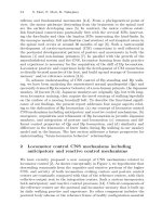
Fig. 1. Variety of possible locomotion of snake robot
2. Inching mode: This is one of the common undulatory movements of ser-
pentine mechanisms. The robot generates a vertical wave-shape using
its units from the rear end and propagates the ’wave’ along its body -
resulting a net advancement in its position.
3. Twisting mode: In this mode the robot mechanism folds certain joints
to generate a twisting motion within its body, resulting in a side-wise
movement [5] .
4. Wheeled locomotion mode: This is one of the common wheeled locomo-
tion mode where the passive wheels (without direct drive) are attached on
the units resulting low friction along the tangential direction of the robot
body line while increasing the friction in the direction perpendicular to
that [2].
5. Bridge mode: In this mode the robot configures itself to ”stand” on its two
end units in a bridge like shape. This mode has the possibility of imple-
mentation of two-legged walking type locomotion. The basic movement
consists of left-right swaying of the center of gravity in synchronism with
by lifting and forwarding one of the supports, like bipedal locomotion.
Motions such as somersaulting may also be some of the possibilities.
The snake robots which have many functions, locomotion modes and 3D mo-
tion have been developed, but in the study of controller design for the snake
robots the movement is restricted to 2D motion. Construction of a controller
which accomplishes 3D motion of 3D snake robots is one of challenging and
important problems.
Chirikijian and Burdick discuss the sidewinding locomotion of the snake
robots based on the kinematic model [6]. Ostrowski and Burdick analyze the
controllability of a class of nonholonomic systems, that the snake robots are
included, on the basis of the geometric approach [7]. The feedback control
law for the snake head’s position using Lyapunov method has been developed
by Prautesch et al. on the basis of the wheeled link model [8]. They point out

the controller can stabilize the head position of the snake robot to its desired
Experimental Study on Control of Redundant 3-D Snake Robot 119
value, but the configuration of it converges to a singular configuration. We
find that introduction of links without wheels and shape controllable points
in the snake robot’s body makes the system redundancy controllable.
In this paper we consider the singular configuration avoidance of the re-
dundant 3D snake robots. Using redundancy, it becomes possible to accom-
plish both the main objective of controlling the position and the posture
of the snake robot head and the sub-objective of the singular configuration
avoidance. Experimental results by using a 13-link snake robot (ACM-R3 [9])
are shown.
2 Redundancy controllable system
In our previous paper we define the redundancy controllable system and
propose structure design methodology of redundant snake robots based on
the wheeled link model [10].
Let q ∈ R
¯n
be the state vector, u ∈ R
¯p
be the input vector, w ≡ Sq ∈ R
¯q
be the state vector to be controlled, S be a selection matrix whose row vec-
tors are independent unit vectors related to generalized coordinates, A(q) ∈
R
¯mׯq
,B(q) ∈ R
¯mׯp
,where ¯m is number of equations. We define that the
system
A(q)

˙
w = B(q)u, u = u
1
+ u
2
(1)
is redundancy controllable if ¯p>¯q (redundancy I), ¯p> ¯m (redundancy II),
1
the matrix A is full column rank, B is full row rank, and following two
conditions are satisfied.
1. There exists an input u
1
which accomplishes the main objective of the
convergence of the vector w to the desired state w
d
(w → w
d
,
˙
w →
˙
w
d
).
2. There exists an input u = u
1
+ u
2
which accomplishes the increase (or
decrease) of a cost function V (q) related to the sub-objective compared to

the input u
1
and does not disturb the main objective.
For a snake robot based on the wheeled link model we discuss the condi-
tion that the system is redundancy controllable [10].
3 Kinematic model of snake robots
Let us consider a redundant n-link snake robot on a flat plane. We introduce
a coordinate frame Σ
A
which is fixed on the head of the snake robot. The tip
point of the snake head is taken as the origin of Σ
A
. The reference configu-
ration is set as a straight line configuration on the ground as shown in Fig.
2. The
A
x axis is set as the central body axis of the snake robot taking the
1
In the case of ¯m =¯p, if the state vector to be controlled
˙
w in (1) is given, the
input u is determined uniquely. In this sense the system is not redundant, so we
introduce the redundancy II.
120 Fumitoshi Matsuno, Kentaro Suenaga
reference configuration. All joints rotate around
y
axis or
z
axis in the ref-
erence configuration. Let

A
ˆ
l
i
=[l
i
, 0, 0]
T
be a link vector from the i-th joint
to the (i − 1)-th joint with respect to Σ
A
in Fig. 2. Let φ
i
be the relative
Fig. 2. Reference configuration of 3D snake robot
joint angle between link i and i +1.Thelinkvector
A
l
i
with respect to Σ
A
is expressed as
A
l
i
= R
φ
1
···R
φ

i−1
A
ˆ
l
i
(i =1, ···,n)(2)
where R
φ
i
is Rot(y, φ
i
)=R
jφ
i
or Rot(z,φ
i
)=R
kφ
i
. The 3D snake robot
divided two parts. One is the base part and the other is the head part. We
define that the first n
h
links (head part) are not contact with the ground,
and the residual n
b
links (base part) are on the same plane which is parallel
to the ground. In the base part wheeled links are contact with the ground.
Let us introduce inertial Cartesian coordinate frame Σ
W

and the coordinate
frame Σ
B
which is fixed on the end point of the base part ((n
h
+ 1)-th link)
as shown in Fig. 3. We introduce following three assumptions.
[assumption 1]: All joints of the base part rotate around z axis.
[assumption 2]: Environment is flat.
[assumption 3]: The robot is supported by the wheels of the base part and
the head part is not contact with the ground.
Fig. 3. Coordinate systems of 3D snake robot
Experimental Study on Control of Redundant 3-D Snake Robot 121
The rotation matrix from Σ
B
to Σ
A
is given as
A
R
B
= R
φ
1
···R
φ
n
h
. (3)
Let ψ be the absolute attitude angle of the head of the base part about z

axis, then the rotation matrix from Σ
B
to Σ is expressed as
W
R
B
= R
kψ
(4)
where R
kψ
= Rot(z,ψ). The rotation matrix
W
R
A
from Σ
A
to Σ is expressed
as
W
R
A
=
W
R
B
(
A
R
B

)
−1
= R
kψ
R
−φ
n
h
···R
−φ
1
. (5)
Using (5) and (2) gives the link vector l
i
with respect to Σ
l
i
= R
kψ
R
−φ
n
h
···R
−φ
i
A
ˆ
l
i

(i =1, ···,n
h
)
l
n
h
+1
= R
kψA
ˆ
l
n
h
+1
l
i
= R
kψ
R
φ
n
h
+1
···R
φ
i
−1
A
ˆ
l

i
(i = n
h
+2, ···,n).
(6)
Let (R, P, Y ) be roll, pitch, yaw angles, then we obtain
R =atan2(±
˜
R
32
, ±
˜
R
33
)
P =atan2(−
˜
R
31
, ±

˜
R
2
11
+
˜
R
2
21

)
Y −ψ =atan2(±
˜
R
21
, ±
˜
R
11
)
(7)
where

R = R
−φ
n
h
···R
−φ
1
. Using (6) and (7) yields
l
i
= R
k(Y −atan2(±
˜
R
21
,±
˜

R
11
))
R
−φ
n
h
···R
−φ
i
A
ˆ
l
i
(i =1, ···,n
h
)
l
n
h
+1
= R
k(Y −atan2(±
˜
R
21
,±
˜
R
11

))A
ˆ
l
n
h
+1
l
i
= R
k(Y −atan2(±
˜
R
21
,±
˜
R
11
))
R
φ
n
h
+1
···R
φ
i
−1
A
ˆ
l

i
(i = n
h
+2, ···,n).
(8)
The middle position P
i
=[x
i
,y
i
,z
i
]
T
of the rotational axis of two wheels
attached on the link i is expressed as
P
i
= P
h
− l
1
− l
2
−···−l
i−1
−
l
wi

l
i
l
i
(9)
where P
h
is the position vector of the snake head and l
wi
is the distance
between the joint i and the attached position of the wheel of the link i.As
the wheel does not slip to the side direction, the velocity constraint condition
should be satisfied. If the i-th link is wheeled and contact with the ground,
the constraint can be written as
˙x
i
sin θ
i
− ˙y
i
cos θ
i
= 0 (10)
122 Fumitoshi Matsuno, Kentaro Suenaga
where θ
i
is the absolute attitude of the i-th link about z-axis and it is ex-
pressed as
θ
i

= ψ +
i−1

j=n
h
+1
φ
j
= Y − atan2(±
˜
R
21
, ±
˜
R
11
)+
i−1

j=n
h
+1
φ
j
. (11)
From the assumption 3 z-element of the position vector of the first link of
the base part is constant. We set it as h, then we obtain
(P
h
− l

1
− l
2
−···−l
n
h
)
T
e
z
= h (12)
where l
z
=[001]
T
. Using time derivative of the geometric relation (7)(9)(12)
and the velocity constraint condition (10) yields kinematic model of 3D snake
robot.
4 Condition for redundancy controllable system
We consider control of position and posture of the snake head. Let w =
[ x
h
y
h
z
h
RP Y]
T
be the vector of the position and the posture of
the snake head, θ =[φ

1
··· φ
n−1
]
T
be the vector of relative joint angles,
q =[w
T
θ
T
]
T
∈ R
n+5
be the generalized coordinates. The angular velocity
of each joint is regarded as the input of the robot system. If a wheel free link
is connected to the tail, the movement of the added link does not contribute
to the movement of the snake head. So we assume that wheel is attached at
the tail link. If all links are wheeled, then we obtain
¯
A(q)
˙
w =
¯
B(q)u , u =
˙
θ (13)
where
¯
A =

⎡
⎢
⎢
⎢
⎢
⎢
⎢
⎢
⎢
⎢
⎣
a
11
a
12
000 a
16
a
21
a
22
000 a
26
.
.
.
.
.
.
.

.
.
.
.
.
.
.
.
.
.
.
a
n
b
1
a
n
b
2
000a
n
b
6
001000
000100
000010
⎤
⎥
⎥
⎥

⎥
⎥
⎥
⎥
⎥
⎥
⎦
¯
B =
⎡
⎢
⎢
⎢
⎢
⎢
⎢
⎢
⎢
⎢
⎣
b
11
··· b
1n
h
0 ··· 0
b
21
··· b
2n

h
−l
w(n
h
+2)
··· 0
.
.
.
.
.
.
.
.
.
.
.
.
b
n
b
1
··· b
n
b
n
h
b
n
b

(n
h
+1)
···−l
wn
b
(n
b
+1)1
···b
(n
b
+1)n
h
0 ··· 0
b
(n
b
+2)1
···b
(n
b
+2)n
h
0 ··· 0
b
(n
b
+3)1
···b

(n
b
+3)n
h
0 ··· 0
⎤
⎥
⎥
⎥
⎥
⎥
⎥
⎥
⎥
⎥
⎦
Experimental Study on Control of Redundant 3-D Snake Robot 123
In (13), the first n
b
equations are obtained from (9) (10), the (n
b
+ 1)-th
from the derivative of (12), and the (n
b
+ 2)-th and (n
b
+ 3)-th equations
from derivative of the first two equations of (7).
Let m be the number of wheeled links of the base part. The kinematic
model is expressed as

A(q)
˙
w = B(q)u , u =
˙
θ (14)
We consider conditions so that the n-link snake robot system can be regarded
as the redundancy controllable system which is defined in the section 2. To
satisfy the redundancy II the inequality
[condition 1] : 3 ≤ m<n− 4
should be satisfied. To satisfy the full row rankness of the matrix B we should
introduce following conditions.
[condition 2] :
In the case that the (n
h
+ 1)-th link is wheel free : n
h
≥ 3
In the case that the (n
h
+ 1)-th link is wheeled : n
h
≥ 4
[condition 3] :
All joints of the head part do not have same direction of rotational axes.
These three conditions are sufficient condition so that the system is redun-
dancy controllable [10].
The necessary and sufficient condition for the existence of the solution of
the system (14) is
rank[A, Bu]=rankA. (15)
5 Controller design for main-objective

Let us define the control input as
u =
˙
θ = B
+
A{
˙
w
d
− K(w −w
d
)}
+(I − B
+
B)k (16)
where B
+
is a pseudo-inverse matrix of B, k is an arbitrary vector and K>0.
The first term of the right side of (16) is the control input term to accomplish
the main objective of the convergence of the state vector w to the desired
value w
d
. As the second term (I − B
+
B)k belongs to the null space of the
matrix B, we obtain
Bu = A{
˙
w
d

− K(w −w
d
)}. (17)
124 Fumitoshi Matsuno, Kentaro Suenaga
As the vector Bu can be expressed as a linear combination of column vectors
of the matrix A, the condition (14) of the existence of the solution (14)
is satisfied. The second term in (16) does not disturb the dynamics of the
controlled vector w. As there is no interaction between w and θ, we find that
the control law (16) accomplishes the sub-objective.
The closed-loop system is expressed as
A{(
˙
w −
˙
w
d
)+K(w −w
d
)} =0. (18)
If the matrix A is full column rank, the uniqueness of the solution is guaran-
teed. The solution of (18) is given as
˙
w −
˙
w
d
+ K(w −w
d
)=0
and we find that the controller ensures the convergence of the controlled state

vector to the desired value (w −→ w
d
). A set of joint angles which satisfies
rankA<q(A is not full column rank) means the singular configuration, for
example a straight line (φ
i
=0,i =1,···,n− 1).
6 Controller design for sub-objective
We consider the controller design for the sub-objective. In the control law
(16), k is an arbitrary vector. Let us introduce the cost function V (q)which
is related to the sub-objective. If we set the vector k as the gradient k
1
of the
cost function V (q) with respect to the vector θ related to the input vector
u, we obtain
k
1
= ∇
θ
V (q)=

∂V
∂θ
1
···
∂V
∂θ
n−1

and we find that the second term of (16) accomplishes the increase of the

cost function V . Actually we can derive
˙
V (q)=(∂V/∂w)
˙
w +(∂V/∂θ)
˙
θ
=(∂V/∂w)
˙
w + k
T
B
+
A{
˙
w
d
−K(w−w
d
)}
+ k
T
1
(I − B
+
B)k
1
. (19)
As I −B
+

B ≥ 0 [11], we find that the second term of the input (16) accom-
plishes the increase of the cost function V .
In the case that the sub-objective is the singularity avoidance, we set
B
+
= B
T
(BB
T
)
−1
and
V = α(det(A
T
A)) + β(det(BB
T
)) (20)
where α, β > 0. The first term of the right side of (20) implies the measure of
the singular configuration. The second term of the right side of (20) is related
to the manipulability of the system.
Experimental Study on Control of Redundant 3-D Snake Robot 125
7 Experiments
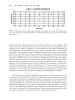
To demonstrate the validity of the proposed control law experiments have
been carried out. The snake robot that we use for the experiments is ACM-
R3 [9] as shown in Fig. 4. The snake robot has 13 links and the 2, 6, 8,
9, 10, 12, 13-th links are wheeled. The length l
i
(i =1, ···, 13) of the links
are as follows: l
1

= l
7
= l
8
= l
9
= l
10
= l
11
= l
12
=0.16[m], l
2
= l
3
=
l
4
= l
5
= l
6
= l
13
=0.08[m]. We set K = I, α =0.2,β =2.0 × 10
6
.The
initial position and posture of the head of the snake robot and initial relative
joint angles are set as w(0) = [0, −0.1, 0.142, 0.0715, −0.143,π/10]

T
,θ(0) =
[0,π/18,π/30,π/18,π/12, −π/9,π/6,π/6, −π/9, −π/6, −π/10,π/30]
T
.
Fig. 4. A research platform robot (ACM-R3)
In experiments, to measure the position and the posture of the snake head
we use Quick MAG IV stereo vision system with two fixed CCD cameras. The
desired trajectory w
d
corresponding to w is represented as the broken lines
in Figs. 5 and 6. Fig. 5 shows the transient responses for the controller (16)
without using redundancy (k = 0). From Fig. 5(a) and (c) we find that
the snake robot can not track the desired head trajectory because of the
convergence to the singular configuration of a straight line. Fig. 6 shows the
transient responses for the controller (16) with using redundancy (k = k
1
).
From Fig. 6 (a) and (c) we find that the snake robot avoids the singular
configuration of the straight line. Experimental results show the effectiveness
of the proposed controller.
8 Conclusion
We have considered control of redundant 3D snake robot based on kinematic
model. We derived conditions so that the snake robot system is redundancy
controllable. We propose controller that the snake head tracks the desired
trajectory and the robot avoids singular configurations by using redundancy.
Experimental results ensure the effectiveness of the proposed control law.
126 Fumitoshi Matsuno, Kentaro Suenaga
0 5 10 15
0

0.5
1
1.5
2
2.5
x
h
, x
hd
[m]
0 5 10 15
0
0.5
1
1.5
2
2.5
y
h
, y
hd
[m]
0 5 10 15
0
0.1
0.2
0.3
z
h
, z

hd
[m]
0 5 10 15
−1
−0.5
0
0.5
1
R , R
d
[rad]
0 5 10 15
−1
−0.5
0
0.5
1
P , P
d
[rad]
t [s]
0 5 10 15
−0.5
0
0.5
1
1.5
Y , Y
d
[rad]

t [s]
(a) w(−−−−)andw
d
(−−−)
0 5 10 15
−1
0
1
u
1
[rad/s]
0 5 10 15
−1
0
1
u
2
[rad/s]
0 5 10 15
−1
0
1
u
3
[rad/s]
0 5 10 15
−1
0
1
u

4
[rad/s]
0 5 10 15
−1
0
1
u
5
[rad/s]
0 5 10 15
−1
0
1
u
6
[rad/s]
0 5 10 15
−1
0
1
u
7
[rad/s]
0 5 10 15
−1
0
1
u
8
[rad/s]

0 5 10 15
−1
0
1
u
9
[rad/s]
0 5 10 15
−1
0
1
u
10
[rad/s]
0 5 10 15
−1
0
1
u
11
[rad/s]
t [s]
0 5 10 15
−1
0
1
u
12
[rad/s]
t [s]

b) Input u
1
, ···,u
12
0 2 4 6 8 10 12 14 16 18
0
0.5
1
1.5
2
det(A
T
A)
0 2 4 6 8 10 12 14 16 18
0
0.5
1
1.5
2
2.5
3
x 10
8
det(BB
T
)
t [s]
(c) det(A
T
A) and det(BB

T
)
Fig. 5. Transient responses for controller without using redundancy (k =0)
Experimental Study on Control of Redundant 3-D Snake Robot 127
0 5 10 15
0
0.5
1
1.5
2
2.5
x
h
, x
hd
[m]
0 5 10 15
0
0.5
1
1.5
2
2.5
y
h
, y
hd
[m]
0 5 10 15
0

0.1
0.2
0.3
z
h
, z
hd
[m]
0 5 10 15
−1
−0.5
0
0.5
1
R , R
d
[rad]
0 5 10 15
−1
−0.5
0
0.5
1
P , P
d
[rad]
t [s]
0 5 10 15
−0.5
0

0.5
1
1.5
Y , Y
d
[rad]
t [s]
(a) w(−−−−)andw
d
(−−−)
0 5 10 15
−1
0
1
u
1
[rad/s]
0 5 10 15
−1
0
1
u
2
[rad/s]
0 5 10 15
−1
0
1
u
3

[rad/s]
0 5 10 15
−1
0
1
u
4
[rad/s]
0 5 10 15
−1
0
1
u
5
[rad/s]
0 5 10 15
−1
0
1
u
6
[rad/s]
0 5 10 15
−1
0
1
u
7
[rad/s]
0 5 10 15

−1
0
1
u
8
[rad/s]
0 5 10 15
−1
0
1
u
9
[rad/s]
0 5 10 15
−1
0
1
u
10
[rad/s]
0 5 10 15
−1
0
1
u
11
[rad/s]
t [s]
0 5 10 15
−1

0
1
u
12
[rad/s]
t [s]
(b) Input u
1
, ···,u
12
0 2 4 6 8 10 12 14 16 18
0
0.5
1
1.5
2
det(A
T
A)
0 2 4 6 8 10 12 14 16 18
0
0.5
1
1.5
2
x 10
8
det(BB
T
)

t [s]
(c) det(A
T
A) and det(BB
T
)
Fig. 6. Transient responses for the controller with using redundancy (k = k
1
)
128 Fumitoshi Matsuno, Kentaro Suenaga
References
1. J. Gray, Animal Locomotion, pp. 166-193, Norton, 1968
2. S. Hirose, Biologically Inspired Robots (Snake-like Locomotor and Manipulator),
Oxford University Press, 1993
3. B. Klaassen and K. Paap, GMD-SNAKE2: A Snake-Like Robot Driven by
Wheels and a Method for Motion Control, Proc. IEEE Int. Conf. on Robotics
and Automation, pp. 3014-3019, 1999.
4. M. Yim, D. Duff and K. Poufas, PolyBot: a Modular Reconfigurable Robot,
Proc. IEEE Int. Conf. on Robotics and Automation, pp. 514-520, 2000.
5. T. Kamegawa, F. Matsuno and R. Chatterjee, Proposition of Twisting Mode
of Locomotion and GA based Motion Planning for Transition of Locomotion
Modes of a 3-dimensional Snake-like Robot, Proc. IEEE Int. Conf. on Robotics
and Automation, pp. 1507-1512, 2002.
6. G. S. Chirikijian and J. W. Burdick, The Kinematics of Hyper-Redundant
Robotic Locomotion, IEEE Trans. on Robotics and Automation, Vol. 11, No.
6, pp. 781-793, 1995
7. J. Ostrowski and J. Burdick, The Geometric Mechanics of Undulatory Robotic
Locomotion, Int. J. of Robotics Research, Vol. 17, No. 6, pp. 683-701, 1998
8. P. Prautesch, T. Mita, H. Yamauchi, T. Iwasaki and G. Nishida, Control and
Analysis of the Gait of Snake Robots, Proc. COE Super Mechano-Systems Work-

shop’99, pp. 257-265, 1999
9. M. Mori and S. Hirose, Development of Active Cord Mechanism ACM-R3 with
Agile 3D Mobility, Proc. IEEE/RSJ Int. Conf. on Intelligent Robots and Sys-
tems, pp. 1552-1557, 2001.
10. F. Matsuno and K. Mogi, Redundancy Controllable System and Control of
Snake Robot with Redundancy based on Kinematic Model, Proc. IEEE Conf.
on Decision and Control, pp. 4791-4796, 2000.
11. Y. Nakamura, H. Hanafusa and T. Yoshikawa, Task-Priority Based Redundancy
Control of Robot Manipulators, Int. J. of Robotics Research , Vol. 6, No. 2, pp.
3-15, 1987
Part 4
Bipedal Locomotion
Utilizing Natural Dynamics
Simulation Study of Self-Excited Walking of a
Biped Mechanism with Bent Knee
Kyosuke Ono and Xiaofeng Yao
Tokyo Institute of Technology, Department of Mechanical and Control
Engineering, 2-12-1 Ookayama, Meguro-ku, Tokyo, Japan 152-8552,

Abstract. This paper presents a simulation study of self-excited walking of a four-
link biped model whose support leg is holding a bending angle at the knee. We found
that the biped model with a bent knee can walk faster than the straight support
leg model that has been studied so far. The convergence characteristics of the self-
excited walking are shown in relation to the bent knee angle. By using standard
link parameter values we investigated the effect of the bent knee angle and foot
radius on walking performance. We found that the walking speed of 0.7 m/s can
be achieved when the bent knee angle is 15 degrees and the foot radius is 40mm.
1 Introduction
Since a biped robot is the ultimate goal of robotic machines in terms of versa-
tility with environments, friendliness to the human society and sophistication

of locomotion, it has been studied by a great number of researchers. In the
first age of research of biped mechanisms or humanoid robots from the 1970s
to 1995, many control strategies of a biped walking were proposed [1-7]. In
addition, dynamic stability of walking locomotion inherent to a biped mech-
anism on a shallow slope were also studied by a number of researchers [8-10]
and passive walking are presented by McGeer [11-13].
At the end of 1995, Honda developed an advanced humanoid robot based
on trajectory planning and zero moment point (ZMP) control [14]. Since
then, the research of humanoid robots have focused on realizing various kinds
of intelligent functions similar to human beings. However, these humanoid
robots consume a high power in spite of slow walking compared with human.
For this reason it will be important to study a biped mechanism that can
perform natural walking in order to improve the walking efficiency.
As a control method of the natural dynamics of the biped mechanism,
Ono et al. proposed a self-excitation control of a 2-degree-of-freedom (2-
DOF) swing leg and showed that a four-link biped mechanism with and
without feet can walk on a level ground by means of only one hip motor in
numerical simulation and experiment [15-16]. In this biped model the stance
leg is assumed to be kept straight by some rock mechanism. Walking speed
can be increased to over 0.4m/s by using a cylindrical foot, but it is still slow
compared with human natural walking.
132 Kyosuke Ono, Xiaofeng Yao
This study aims to find principles of fast biped walking with high efficiency
based on self-excitation. Through our understanding of human walking pat-
terns, we know that people always retain some knee flexion during walking
[17] when we want to walk fast. Therefore, we try to apply a bent knee angle
to the support leg in order to make it walk faster.
In the next section, the analytical model and its basic equations of loco-
motion will be introduced. In section 3, we show the typical simulated results
of stable biped locomotion on level ground with and without a bent knee

angle and foot and the convergence characteristics of the self-excited walking
in relation to the bent angle. Next, we present the calculated results of the
effect of the knee bent angle with and without a foot radius on the walking
performance.
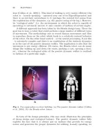
2 The analytical model and basic equations
Figure 1 shows the biped mechanism that walks with a bent knee. We consider
the biped walking motion on a sagittal plane. The biped model consists of
only two legs and does not have a torso. The two legs are connected in a series
at the hip joint through a motor. Both legs have a thigh and a shank that
are connected at the knee joint. We assume that the biped has knee brakes
so that the knee can be locked at any bent angle after the knee collision of
the swing leg. The support leg does not extend fully but retains some flexion
during the stance phase. Therefore the brake is activated before the swing leg
becomes straight and keeps a desired knee angle between the thigh and the
shank. The brake is released just when the supporting leg enters the swing
phase.
Fig. 1. Self-excited mechanism with bent knee and cylindrical foot
Simulation Study of Self-Excited Walking of a Biped Mechanism 133
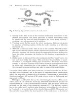
Fig. 2. Two phases of biped walking
Figure 2 shows the algorithm of biped walking. Biped walking can be
divided into two phases: the swing leg phase and the touch down phase,
1. From the start of the swinging leg motion to the lock of the knee joint
of the swinging leg by the brake. In this phase, only the brake of the
supporting leg is activated.
2. From the lock of the knee joint of the swinging leg to the touch down of
the bent swinging leg. In this phase, the brakes of both legs are activated.
We assume that the change of the supporting leg to the swinging leg occurs
instantly and the friction force between the foot and the ground is large
enough to prevent a slip.
To realize stable biped walking on a level ground, the swinging leg should

bend at the knee to prevent the tip from touching the ground. In addition, the
energy dissipated through knee and foot collisions and joint friction should be
supplied by the motor. The swing leg motion can be autonomously generated
by the asymmetrical feedback of the form,
T
2
= −kθ
3
(1)
If the feedback gain k is increased to a certain value, the swing leg motion
begins to be self-excited and the kinetic energy of the swinging leg increases.
Since the swing motion has a constant period at any swing amplitude, there is
an angular velocity of the support leg whose swing motion as an inverted pen-
dulum can synchronize with the swing leg motion. This velocity determines
the walking speed.
134 Kyosuke Ono, Xiaofeng Yao
In addition, the synchronized motion between the inverted pendulum mo-
tion of the supporting leg and the two-DOF pendulum motion of the swinging
leg, as well as the balance of the input and the output energy, should have
stable characteristics against small deviations from the synchronized motion.
Fig. 3. Analyical model of three degree of freedom walking mechanism
It is also assumed that a small viscous rotary damper with coefficient γ
3
is applied to the knee joint of the swing leg, which produces a torque as:
T
3
= −γ
3
(
˙

θ
3
−
˙
θ
2
)(2)
Under the assumption of a fixed bent knee angle of the supporting leg and
a free knee joint of the swinging leg, the analytical model during the first
phase is treated as a three-DOF link system, as shown in Fig.3. We get the
equation of motion in the first phase as:
⎡
⎣
M1
11
M1
12
M1
13
M1
22
M1
23
sym M1
33
⎤
⎦
⎡
⎣
¨

θ
1
¨
θ
2
¨
θ
3
⎤
⎦
+
⎡
⎣
0 C1
12
C1
13
−C1
12
0 C1
23
−C1
13
−C1
23
0
⎤
⎦
⎡
⎣

˙
θ
2
1
˙
θ
2
2
˙
θ
2
3
⎤
⎦
+
⎡
⎣
K1
1
K1
2
K1
3
⎤
⎦
=
⎡
⎣
−T
2

T
2
− T
3
−T
3
⎤
⎦
(3)
where the elements M 1
ij
,C1
ij
and K1
i
of the matrices are shown in Ap-
pendix 1. T
2
is the feedback input torque given by Eq.(1) while T
3
is the
viscous resistance torque at the knee joint, which is given by Eq.(2).
Simulation Study of Self-Excited Walking of a Biped Mechanism 135
When the angle between the shank and thigh of the swing leg becomes a
certain value, the brake is activated and locks the knee joint. This signifies
the end of the first phase. We assume the knee collision occurs plastically at
this time. From the assumption of conservation of momentum and angular
momentum before and after the knee collision, angular velocities after the
knee collision are calculated from the condition
˙

θ
+
2
=
˙
θ
+
3
, and the equation
is written as:
⎡
⎣
˙
θ
+
1
˙
θ
+
2
˙
θ
+
3
⎤
⎦
=[M ]
−1
⎡
⎣

f
1
(θ
1
,
˙
θ
−
1
)
f
2
(θ
2
,θ
−
2
) − τ
f
3
(θ
3
,θ
−
3
)+τ
⎤
⎦
(4)
where the elements of the matrix[M ] are the same as M1

ij
in Eq.(3). f
1
,f
2
and
f
3
are presented in Appendix 2. τ is the impulse moment at the knee.
During the second phase, the biped system can be regarded as a two-DOF
link system. The basic equation becomes

M2
11
M2
12
M2
12
M2
22

¨
θ
1
¨
θ
2

+


0 C2
12
−C2
12
0

˙
θ
1
˙
θ
2

+

K2
1
K2
2

=0 (5)
where the elements M2
ij
,C2
ij
and K2
ij
of the matrices are shown in Ap-
pendix 3.
We assume that the collision of the swinging leg with the ground occurs

un-elastically and the friction between the foot and the ground is large enough
to prevent slipping. Just like knee collision, the angular velocities of the links
after the collision can be derived from conservation laws of momentum and
angular momentum. At this time, τ = 0 is put into Eq.(4). After the collision,
the supporting leg turn to the swinging leg immediately and the system enter
the first phase again.
Table 1 . Link parameter values used for simulation
Parameters Thigh Shank Leg
Length l
i
[m] 0.4 0.4 0.8
Mass n
i
[kg] 2.0 2.0 4.0
Center of mass a
i
[m] 0.2 0.2 0.4
Moment of inertia at mass center I
i
[kgm
2
] 0.027 0.027 0.21
3 The results of simulation
The values of the link parameters used in the simulation are shown in Table
1. We use the same values as in our preceding paper [15] because it is easy
to find the influence of the bent knee angle by comparing the two results.
The fourth order Runge-Kutta method was used to numerically solve the
136 Kyosuke Ono, Xiaofeng Yao
basic equations. In order to increase the accuracy, the time step is set to be
1ms. Regarding the effect of viscous rotary damper γ

3
, it is found that a
proper value will yield the phase delay of the shank. This helps to increase
the foot clearance. By considering the efficiency, γ
3
=0.15 Nms/rad is used
in the simulation. In the numerical simulation, steady walking locomotion
is obtained with bent knee angles of less than 17 degrees. When the angle
is larger than 17 degrees, the step length decreases suddenly and the biped
mechanism falls forward.
Figure 4 illustrates the stick figures of the stable self-excited walking gaits
during four steps (two walking cycles) under the conditions of when the model
has the bent knee angle and foot or not. For the convenience of comparison,
the feedback gain k is set to be 8Nm/rad in all the cases. In Fig.4 (a), the
biped has no bent knee angle and no foot. The step length is 0.18 m and the
period of one step is 0.64 s, so the walking velocity is 0.28 m/s. In Fig.4 (b),
10 degrees of the bent knee angle is added to the support leg. The step length
increases to 0.31 m and the period decreases a little, so that the velocity is
increased to 0.5 m/s. The velocity increase is mainly caused by the increase
in the moment to drive the supporting leg forward due to the forward shift
of the mass center of the leg. In Fig.4 (c), the velocity is increased further to
0.65 m/s by giving the model a foot whose radius R is 0.3 m. From the stick
figures, we can clearly observe the increase of the walking speed. We also
note that the shank motion of the swing leg delays from the thigh motion
that yields a foot clearance (the height of the tip of the swing leg from the
ground) for stable walking.
The initial start condition of the supporting leg that can lead to stable
walking and the typical converging process of the self-excited walking are
shown in Fig. 5 when the knee angle αgs zero and the feedback gain k is
6 Nm/rad. Figure 5(a) shows the initial start angle and angular velocity of

the supporting leg that can converge to a limit cycle of walking motion and
the converging processes from the three different initial conditions of 1 to 3.
This graph shows the basin of a limit cycle on a Poincare phase plane at the
start of a swing of the supporting leg. The star symbol indicates the start
condition of the supporting leg in the steady walking motion (limit cycle). We
note that the same unique start condition of the limit cycle can be obtained
from three different initial conditions that are far apart from each other.
Figure 5(b) shows the change of step length as a function of time in the
converging process from the three different initial conditions corresponding
to those in Fig.5(a). Since the walking period is 1.3 seconds, as will be shown
later, steady walking can be achieved after about ten cycles of walking.
α =0
◦
R =0mα =10
◦
R =0mα =10
◦
R =0.3m
Figure 6 shows the change of the stable start condition when the bent knee
angle is changed to 5, 10 and 15 degrees. We note from these figures that
stable walking becomes difficult as the bent knee angle increases when the
mass distribution of the biped has not changed. The straight line on the main
Simulation Study of Self-Excited Walking of a Biped Mechanism 137
Fig. 4. Stick figures duringin two walking cycles
trunk of the basin is calculated from the synchronizing condition between
the supporting leg and swinging leg based on a physical model, although
not explained in detail. A good agreement between the line and calculated
point of the stable start condition indicates that stable self-excited walking is
generated when the swing leg motion and the support leg motion synchronize
with each other

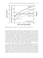
Figure 7 shows the effect of the bent knee angle on the walking velocity,
input power, specific cost, step length and period respectively when k=8
Nm/rad and R=0 m. The average input power is calculated by:
P =
1
t
end

t
end
0



˙
θ
2
kθ
3



dt (6)
The specific cost is defined as:
E =
P
mgV
(7)
From Fig. 7 we note that as the bent angle increases, the step length increases,
the period decrease and then the walking velocity increases. It should be

noted that the walking velocity at α = x6 increases by 2.3 times that at
α=0, whereas the increased rate in specific cost is 1.4. The reason for this
is considered as follows: As the bent knee angle increases, the position of
the mass center of the swing leg approaches the hip joint. Therefore, the
swing period will decrease. At the same time, the center of mass is moved
138 Kyosuke Ono, Xiaofeng Yao
Fig. 5. Start angular position and velocity of support leg that can converge
to a limit cycle of walking and converging processes from three different initial
conditions(α = 0).(a)Start angular position and velocity of support leg that result
in a limit cycle of walking and converging processes from three different start con-
ditions.(b)Converging processes of step length from three different start conditions.
Fig. 6. Start angular position and velocity of support leg that can result in a stable
walking for various values of bent knee angles
forward in contrast to that of the straight leg. Therefore, the supporting leg
rotates forward faster than in the straight leg model because the offset of
mass yields the gravity torque to make the support leg rotate in the forward
direction. With a shorter swing period and a longer step length, faster walking
is realized in the simulation. However, the specific cost increases until bent
knee angle αreaches 8 degrees because of the rapid increase of input power.
When α>8
◦
the specific cost stops to increase and even decreases a little
because the increase in velocity is faster than the increase in input power.
Since the input torque at the hip joint is proportional to the angle of linkage
3andθ
3
is larger in the bent-knee mode than in the straight-leg mode, the
input power increases when the bent angle increases.
Although not shown here, we also found the influence of feedback gain
on the walking motion. As the feedback gain increases from 7 Nm/rad to 8

Nm/rad, the step length increases a little but the period increases notably