Artificial Mind System – Kernel Memory Approach - Tetsuya Hoya Part 7 pdf
Bạn đang xem bản rút gọn của tài liệu. Xem và tải ngay bản đầy đủ của tài liệu tại đây (570.39 KB, 20 trang )
46 3 The Kernel Memory Concept
(Sound)
w
23
13
w
3k
w
(Image)
c
c
2
x
1
c
3
2
3
K
K
1
K
1
x
2
Fig. 3.6. Example2–abi-directionalMIMOsystemrepresentedbykernelmemory;
in the figure, each of the three kernel units receives and yields the outputs, represent-
ing the bi-directional flows. For instance, when both the two modality-dependent
inputs x
1
and x
2
are simultaneously presented to the kernel units K
1
and K
2
,re-
spectively, K
3
may be subsequently activated via the transfer of the activations from
K
1
and K
2
, due to the link weight connections in between (thus, feedforward ). In re-
verse, the excitation of the kernel unit K
3
can cause the subsequent activations from
K
1
and K
2
via the link weights w
12
and w
13
(i.e. feedback ). Note that, instead of
ordinary outputs, each kernel is considered to output its template (centroid) vector
in the figure
formation (i.e. related to the concept formation; to be described in Chap. 9).
Thus, the information flow in this case is feedforward:
x
1
, x
2
→ K
1
,K
2
→ K
3
.
In contrast, if such a “Gestalt” kernel K
3
is (somehow) activated by the
other kernel(s) via w
3k
and the activation is transferred back to both kernels
K
1
and K
2
via the respective links w
13
and w
23
, the information flow is, in
turn, feedback , since
w
3k
→ K
3
→ K
1
,K
2
.
Therefore, the kernel memory as in Fig. 3.6 represents a bi-directional MIMO
system.
As a result, it is also possible to design the kernel memory in such a way
that the kernels K
1
and K
2
eventually output the centroid vector c
1
and c
2
,
respectively, and if the appropriate decoding mechanisms for c
1
and c
2
are
given (as external devices), we could even restore the complete information
(i.e. in this example, this imitates the mental process to remember both the
sound and facial image of a specific person at once).
Note that both the MIMO systems in Figs. 3.5 and 3.6 can in principle
be viewed as graph theoretic networks (see e.g. Christofides, 1975) and the
3.3 Topological Variations in Terms of Kernel Memory 47
(Input)
. . .
. . .
(Output)
. . .
.
.
.
x
1
2
x
x
3
.
.
.
1
o
2
o
1
y
o
K ( )
2
y
o
K ( )
N
o
N
o
x
1
2
x
1
1
x
1
2
K
2
K ( )
K ( )
c
2
c
1
c
1
c
1
1
2
3
2
1
K ( )
x
1
3
K ( )
1
3
1
o
y
o
K ( )
x
M
Fig. 3.7. Example 3 – a tree-like representation in terms of a MIMO kernel memory
system; in the figure, it can be considered that the kernel unit K
2
plays a role for the
concept formation, since the kernel does not have any modality-dependent inputs
detailed discussion of how such directional flows can be realised in terms of
kernel memory is left to the later subsection “3) Variation in Generating Out-
puts from Kernel Memory: Regulating the Duration of Kernel Activations”
(in Sect. 3.3.3).
Other Representations
The bi-directional representation as in Fig. 3.6 can be regarded as a simple
model of concept formation (to be described in Chap. 9), since it can be
seen that the kernel network is an integrated incoming data processor as well
as a composite (or associative) memory. Thus, by exploiting this scheme,
more sophisticated structures such as the tree-like representation in Fig. 3.7,
which could be used to construct the systems in place of the conventional
symbol-based database, or lattice-like representation in Fig. 3.8, which could
model the functionality of the retina, are possible. (Note that, the kernel
K
2
illustrated around in the centre of Fig. 3.7, does not have the ordinary
modality-dependent inputs, i.e. x
i
(i =1, 2, ,M), as this kernel plays a role
for the concept formation (in Chap. 9), similar to the kernel K
3
in Fig. 3.6.)
3.3.2 Kernel Memory Representations
for Temporal Data Processing
In the previous subsection a variant of network representations in terms of
kernel memory has been given. However, this has not taken into account the
48 3 The Kernel Memory Concept
.
.
.
.
.
.
(Input) (Output)
. . .
. . .
. . .
x
2
1
x
x
M
1
o
2
o
1
y
o
K ( )
2
y
o
K ( )
M
o
x
1
1
x
1
2
x
1
2
x
2
2
x
2
xx
2
x
1
N
N
M
MM
.
.
.
.
.
.
.
.
.
y
o
K ( )
M
M
K ( )
MM
K ( ) K ( )
22
K ( )K ( )
2
K ( )
1
K ( )
1
K ( ) x
1
N
1
K ( )
Fig. 3.8. Example 4 – a lattice-like representation in terms of MIMO kernel memory
system
functionality of temporal data processing. Here, we consider another variation
of the kernel memory model within the context of temporal data processing.
In general, the connectionist architectures as used in pattern classification
tasks take only static data into consideration, whereas the time delay neural
network (TDNN) (Lang and Hinton, 1988; Waibel, 1989) or, in a wider sense
of connectionist models, the adaptive filters (ADFs) (see e.g. Haykin, 1996)
concern the situations where both the input pattern and corresponding output
are varying in time. However, since they still resort to a gradient-descent type
algorithm such as least mean square (LMS) or BP for parameter estimation, a
flexible reconfiguration of the network structure is normally very hard, unlike
the kernel memory approach.
Now, let us turn back to temporal data processing in terms of kernel mem-
ory: suppose that we have collected a set of single domain inputs
11
obtained
during the period of (discrete) time P (written in a matrix form):
X(n)=[x(n), x(n −1), ,x(n −P + 1)]
T
(3.23)
where x(n)=[x
1
(n),x
2
(n), ,x
N
(n)]
T
. Then, considering the temporal vari-
ations, we may use a matrix form, instead of vector, within the template data
11
The extension to multi-domain inputs is straightforward.
3.3 Topological Variations in Terms of Kernel Memory 49
stored in each kernel, and, if we choose a Gaussian kernel , it is normally
convenient to regard the template data in the form of a template matrix (or
centroid matrix in the case of a Gaussian response function) T ∈
N×P
,
which covers the period of time P :
T =
t
1
t
2
.
.
.
t
N
=
t
1
(1) t
1
(2) t
1
(P )
t
2
(1) t
2
(2) t
2
(P )
.
.
.
.
.
.
.
.
.
.
.
.
t
N
(1) t
N
(2) t
N
(P )
(3.24)
where the column vectors contain the temporal data at the respective time
instances up to the period P .
Then, it is straightforward to generalise the kernel memory that employs
both the properties of temporal and multi-domain data processing.
3.3.3 Further Modification
of the Final Kernel Memory Network Outputs
With the modifications of the temporal data processing as described in
Sect. 3.3.2, we may accordingly redefine the final outputs from kernel mem-
ory. Although many such variations can be devised, we consider three final
output representations which are considered to be helpful in practice and can
be exploited e.g. for describing the notions related to mind in later chapters.
1) Variation in Generating Outputs from Kernel Memory:
Temporal Vector Representation
One of the final output representations can be given as a time sequence of the
outputs:
o
j
(n)=[o
j
(n),o
j
(n −1), ,o
j
(n −
ˇ
P + 1)]
T
(3.25)
where each output is now given in a vector form as o
j
(n)(j =1, 2, ,N
o
)
(instead of the scalar output as in Sect. 3.2.4) and
ˇ
P ≤ P . This representa-
tion implies that not all the output values obtained during the period P are
necessarily used, but partially, and that the output generation(s) can be asyn-
chronous (in time) to the presentation of the inputs to the kernel memory. In
other words, unlike conventional neural network architectures, the timing of
the final output generation from kernel memory may differ from that of the
input presentation, within the kernel memory context.
Then, each element in the output vector o
j
(n) can be given, e.g.
o
j
(n) = sort(max(θ
ij
(n))) (3.26)
where the function sort(·) returns the multiple values given to the function
sorted in a descending order, i denotes the indices of all the kernels within a
specific region(s)/the entire kernel memory, and
50 3 The Kernel Memory Concept
θ
ij
(n)=w
ij
K
i
(x(n)) . (3.27)
The above variation in (3.26) does not follow the ordinary “winner-takes-
all” strategy but rather yields multiple output candidates which could, for
example, be exploited for some more sophisticated decision-making processing
(i.e. this is also related to the topic of thinking; to be described later in Chaps.
7 and 9).
2) Variation in Generating Outputs from Kernel Memory:
Sigmoidal Representation
In contrast to the vector form in (3.25), the following scalar output o
j
can
also be alternatively used within the kernel memory context:
o
j
(n)=f(θ
ij
(n)) (3.28)
where the activations of the kernels within a certain region(s)/the entire mem-
ory θ
ij
(n)=[θ
ij
(n),θ
ij
(n−1), ,θ
ij
(n−P +1)]
T
and the cumulative function
f(·) is given in a sigmoidal (or “squash”) form, i.e.
f(θ
ij
(n)) =
1
1 + exp(−b
P −1
k=0
θ
ij
(n −k))
(3.29)
where the coefficient b determines the steepness of the sigmoidal slope.
An Illustrative Example of Temporal Processing – Representation
of Spike Trains in Terms of Kernel Memory
Note that, by exploiting the output variations given in (3.25) or (3.29), it is
possible to realise the kernel memory which can be alternative to the TDNN
(Lang and Hinton, 1988; Waibel, 1989) or the pulsed neural network (Dayhoff
and Gerstein, 1983) models, with much more straightforward and flexible re-
configuration property of the memory/network structures.
As an illustrative example, consider the case where a sparse template ma-
trix T of the form (3.24) is used with the size of (13 × 2), where the two
column vectors t
1
and t
2
are given as
t
1
=[20000.500010001]
t
2
=[2120000010.5100],
i.e. the sequential values in the two vectors depicted in Fig. 3.9 can be used
to represent the situation where a cellular structure gathers for the period of
time P (= 13) and then stores the patterns of spike trains coming from other
neurons (or cells) with different firing rates (see e.g. Koch, 1999).
Then, for instance, if we choose a Gaussian kernel and the overall synap-
tic inputs arriving at the kernel memory match the stored spike pattern to
3.3 Topological Variations in Terms of Kernel Memory 51
12345678910111213
12
3
4
56789
1
0
11 12 1
3
:
1
t
:
2
t
Fig. 3.9. An illustrative example: representing the spike trains in terms of the sparse
template matrix of a kernel unit for temporal data processing (where each of the
two vectors in the template matrix contains a total of 13 spikes)
a certain extent (i.e. determined by both the threshold θ
K
and radius σ,as
described earlier), the overall excitation of the cellular structure (in terms of
the activation from a kernel unit) can occur due to the stimulus and subse-
quently emit a spike (or train) from itself.
Thus, the pattern matching process of the spike trains can be modelled
using a sliding window approach as in Fig. 3.10; the spike trains stored within
a kernel unit in terms of a sparse template (centroid) matrix are compared
with the input patterns X(n)=[x
1
(n) x
2
(n)] at each time instance n.
3) Variation in Generating Outputs from Kernel Memory:
Regulating the Duration of Kernel Activations
The third variation in generating the outputs from kernel memory is due to
the introduction of the decaying factor for the duration of kernel excitations.
For the output generation of the i-th kernel, the following modification can
be considered:
K
i
(x,n
i
) = exp(−κ
i
n
i
)K
i
(x) (3.30)
where n
i
12
denotes the time index for describing the decaying activation of K
i
and the duration of the i-th kernel output is regulated by the newly introduced
factor κ
i
, which is hereafter called activation regularisation factor. (Note that
the time index n
i
is used independent of the kernels, instead of the unique
index n, for clarity.) Then, the variation in (3.30) indicates that the activation
of the kernel output can be decayed in time.
In (3.30), the time index n
i
is reset to zero, when the kernel K
i
is activated
after a certain interval from the last series of activations, i.e. the period of time
when the following relation is satisfied (i.e. the counter relation in (3.12)):
K
i
(x
i
,n
i
) <θ
K
(3.31)
12
Without loss of generality, here the time index n
i
is again assumed to be discrete;
the extension to continuous time representation is straightforward.
52 3 The Kernel Memory Concept
:
2
x
:
1
x
:
1
t
:
2
t
n−12
n−12
n−1 n
nn−1
Input Data to Kernel Unit (Sliding Window)
. . .
. . .
(Pattern Matching)
Template Matrix
Fig. 3.10. Illustration of the pattern matching process in terms of a sliding window
approach. The spike trains stored within a kernel unit in terms of a sparse template
matrix are compared with the current input patterns X(n)=[x
1
(n) x
2
(n)] at each
time instance n
3.3.4 Representation of the Kernel Unit Activated
by a Specific Directional Flow
In the previous examples of the MIMO systems as shown in Figs. 3.5–3.8, some
of the kernel units have (mono-/bi-)directional connections in between. Here,
we consider the kernel unit that can be activated when a specific directional
flow occurs between a pair of kernel units, by exploiting both the notation
of the template matrix as given in (3.24) and modified output in (3.30) (the
fundamental principle of which is motivated by the idea in Kinoshita (1996)).
3.3 Topological Variations in Terms of Kernel Memory 53
K
B
K
A
(A B)
K
B
K
A
(A B)
K
AB
(B A)
K
B
K
A
(A B)
K
B
(A B)
K
A
x
A
(n)
x
B
(n)
x
A
(n)
x
B
(n)
x
A
(n) x
B
(n)x
B
(n)
x
A
(n)
K
BA
K
AB
Fig. 3.11. Illustration of both the mono- (on the left hand side) and bi-directional
connections (on the right hand side) between a pair of kernel units K
A
and K
B
(cf.
the representation in Kinoshita (1996) on page 97); in the lower part of the figure,
two additional kernel units K
AB
and K
BA
are introduced to represent the respective
directional flows (i.e. the kernel units that detect the transfer of the activation from
one kernel unit to the other): K
A
→ K
B
and K
B
→ K
A
Fig. 3.11 depicts both the mono- (on the left hand side) and bi-directional
connections (on the right hand side) between a pair of kernel units K
A
and
K
B
(cf. the representation in Kinoshita (1996) on page 97).
In the lower part of the figure, two additional kernel units K
AB
and K
BA
are introduced to represent the respective directional flows (i.e. the kernel
units that detect the transfer of the activation from one kernel unit to the
other): K
A
→ K
B
and K
B
→ K
A
.
Now, let us firstly consider the case where the template matrix of both the
kernel units K
AB
and K
BA
is composed by the series of activations from the
two kernel units K
A
and K
B
, i.e.:
T
AB/BA
=
t
A
(1) t
A
(2) t
A
(p)
t
B
(1) t
B
(2) t
B
(p)
(3.32)
54 3 The Kernel Memory Concept
where p represents the number of the activation status from time n to n−p+1
to be stored in the template matrix and the element t
i
(j)(i:AorB,j =
1, 2, ,p) can be represented using the modified output given in (3.30) as
13
t
i
(j)=K
i
(x
i
,n− j +1) , (3.33)
or, alternatively, the indicator function
t
i
(j)=
1; ifK
i
(x
i
,n− j +1)≥ θ
K
0 ; otherwise
(3.34)
(which can also represent a collection of the spike trains from two neurons.)
Second, let us consider the situation where the activation regularisation
factor of one kernel unit K
A
,say,κ
A
satisfies the relation:
κ
A
<κ
B
(3.35)
so that, at time n, the kernel K
B
is not activated, whereas the activation of
K
A
is still maintained. Namely, the following relations can be drawn in such
a situation:
K
A
(x
A
(n −p
d
+ 1)) ,K
B
(x
B
(n −p
d
+ 1)) ≥ θ
K
K
A
(x
A
(n)) ≥ θ
K
K
B
(x
B
(n)) <θ
K
(3.36)
where p
d
is a positive value. (Nevertheless, due to the relation (3.35) above, it
is considered that the decay in the activation of both the kernel units K
A
and
K
B
starts to occur at time n, given the input data.) Figure 3.12 illustrates an
example of the regularisation factor setting of the two kernel units K
A
and
K
B
as in the above and the time-wise decaying curves. (In the figure, it is
assumed that p
d
=4andθ
K
=0.7.)
Then, if p
d
<p, and, using the representation of the indicator function
given by (3.34), for instance, the matrix
T
AB
=
011110
001111
(3.37)
can represent the template matrix for the kernel unit K
AB
(i.e. in this case,
p =6andp
d
= 4) and hence the directional flow of K
A
→ K
B
, since the
matrix representation describes the following asynchronous activation pattern
between K
A
and K
B
:
1) At time n −5, neither K
A
nor K
B
is activated;
2) At time n −4, the kernel unit K
A
is activated (but not K
B
);
13
Here, for convenience, a unique time index n is considered for all the kernels in
Fig. 3.11, without loss of generality.
3.3 Topological Variations in Terms of Kernel Memory 55
0 2 4 6 8 10
0
0.2
0.4
0.6
0.8
1
n
K
A
(n)
0 2 4 6 8 10
0
0.2
0.4
0.6
0.8
1
n
K
B
(n)
θ
K
θ
K
Fig. 3.12. Illustration of the decaying curves exp(−κ
i
×n)(i: A or B) for modelling
the time-wise decaying activation of the kernel units K
A
and K
B
; κ
A
=0.03, κ
B
=
0.2, p
d
=4,andθ
K
=0.7
3) At time n −3, the kernel unit K
B
is then activated;
4) The activation of both the kernel units K
A
and K
B
lasts till the time
n −1;
5) Eventually, due to the presence of the decaying factor κ
B
, the kernel
unit K
B
is not activated at time n.
In contrast to (3.37), the matrix (with inverting the two row vectors in
(3.37))
T
BA
=
001111
011110
(3.38)
represents the directional flow of K
B
→ K
A
and thus the template matrix of
K
BA
.
Therefore, provided a Gaussian response function (with appropriately
given the radius, as defined in (3.8)) is selected for either the kernel unit
K
AB
or K
BA
, if the kernel unit receives a series of the lasting activations
from K
A
and K
B
as the inputs (i.e. represented in spiky trains), and the
activation patterns are close to those stored as in (3.37) or (3.38), the kernel
units can represent the respective directional flows.
A Learning Strategy to Obtain the Template Matrix
for Temporal Representation
When the asynchronous activation between K
A
and K
B
occurs and provided
that p = 3 (i.e. for the kernel unit K
AB
/K
BA
), one of the following patterns
56 3 The Kernel Memory Concept
can be obtained using the indicator function representation of the spike trains
by (3.34):
K
A
(x
A
(n)): ··· 0 100000···
K
B
(x
B
(n)): ··· 0 000010···
In the above, it is not sufficient to represent the asynchronous activation
pattern by K
AB
(or K
BA
).
It is then considered that there are two alternative ways to adjust the
template matrix for the kernel unit K
AB
(or K
BA
) that can represent the
asynchronous activation pattern between the kernel units K
A
and K
B
:
1. Adjust the size of the template matrix T
AB
(i.e. varying the factor
p; in this case, assuming that κ
i
= κ
init
(∀i)) ;
2. Update the activation regularisation factors for both the kernel
units K
A
and K
B
For the former, if we increase the number of columns of the template ma-
trix p, until the activation from K
A
and K
B
appears in both the rows (i.e.
p = 5):
K
A
(x
A
(n)): ··· 0 100000 ···
K
B
(x
B
(n)): ··· 0 000010 ···
the asynchronous activation pattern can be represented by the template ma-
trix, i.e.
T
AB
=
10000
00001
(3.39)
An Alternative Learning Scheme – Updating
the Activation Regularisation Factors
Alternatively, the asynchronous activation pattern between K
A
and K
B
can
be represented by updating the activation regularisation factors for both the
kernel unit K
A
and K
B
, without varying p: provided that the regularisation
factor for all the kernel units are initially set as κ
i
= κ
init
(where κ
init
is a
certain positive constant), we update the activation regularisation factors for
both the kernel unit K
A
and K
B
, i.e. κ
A
and κ
B
. Then, we may resort to the
following updating rule:
3.4 Chapter Summary 57
[Updating Rule for the Activation Regularisation
Factor κ
i
]
1) Initially, set κ
i
= κ
init
(∀i).
2)
• For a certain period of time, if the kernel unit K
i
has
activated repetitively, update its regularisation factor
κ
i
as:
κ
i
=
κ
i
− δκ
1
;ifκ
i
>κ
min
κ
min
; otherwise
(3.40)
• In contrast, for a certain period of time, if there is no
activation from K
i
, increase the value of κ
i
:
κ
i
= κ
i
+ δκ
2
(3.41)
in the above where κ
min
(≥ 0) is the minimum value for the regularisation
factor, and δκ
1
and δκ
2
are its decremental and incremental adjustment factor,
respectively.
For instance, if the duration of activation from K
A
becomes longer and,
accordingly, if we successfully obtain the following pattern using the scheme
similar to the above
K
A
(x
A
(n)): ··· 0111000 ···
K
B
(x
B
(n)): ··· 0000010 ···
the template matrix (i.e. p =3)
T
AB
=
100
001
(3.42)
can represent the asynchronous activation of K
A
→ K
B
.
The above scheme can be applied, under the assumption that the duration
of activation K
A
can be different from that of K
B
by varying κ
A
/κ
B
.
Nevertheless, the directed conections also have to be established within
the context of general learning (to be described in Chap. 7). In later chap-
ters, it will then be discussed how the principle of the directed connections
between the kernel units is exploited further and can significantly enhance the
utility for modelling various notions related to artificial mind system, e.g. the
thinking, language, and the semantic networks/lexicon module.
3.4 Chapter Summary
In this chapter, a novel kernel memory concept has been described, which can
subsume conventional connectionist principles.
58 3 The Kernel Memory Concept
The fundamental principle of kernel memory concept is pretty simple;
the kernel memory comprises of multiple kernel units and their link weights
which only represent the strengths of the connections in between. Within the
kernel memory principle, the following three types of kernel units have been
considered:
1) A kernel unit which has both the input and template vector (i.e. the
centroid vector in the case of a Gaussian kernel function) and generates
the output, according to the similarity of the two vectors. (However, as
described in the next chapter, it is also possible to consider the case where
the activation can be due to the transfer of the activations from other
kernel units connected via the link weights, as given by (4.3) or (4.4), to
be described later).
2) A kernel unit functioning similar to the above, except that the input vector
is merely composed of the activations from other kernel units (i.e. as the
neurons in the conventional ANNs). (However, for this type, it still is
possible that the input vector consists of both the activations from other
kernels and the regular input data.)
3) A kernel unit which represents a symbolic node (as in the conventional
connectionist model, or the one with a kernel function given by (3.11)).
This sort of kernel unit is useful in practice, e.g. to investigate the in-
termediate / internal states of the kernel memory. In pattern recognition
problems, for instance, these nodes are exploited to tell us the recognition
results. This issue will be furtherly discussed within a more global context
of target responses in Chap. 7 (Sect. 7.5).
Then, within the kernel memory concept, any rule can be developed to
establish the link weight connections between a pair of kernel units, without
directly affecting the contents of the memory.
In the next chapter, as a pragmatic example, the properties of the kernel
memory concept are exploited to develop a self-organising network model, and
we will see how such a kernel network behaves.
4
The Self-Organising Kernel Memory (SOKM)
4.1 Perspective
In the previous chapter, various topological representations in terms of the
kernel memory concept have been discussed together with some illustrative
examples. In this chapter, a novel unsupervised algorithm to train the link
weights between the KFs is given by extending the original Hebb’s neuropsy-
chological concept, whereby the self-organising kernel memory (SOKM)
1
is
proposed.
The link weight adjustment algorithm does not involve any gradient-
descent type numerical approximation (or the so-called “delta rule”) as in the
conventional approaches, but simply varies the strength of the connections
between KFs according to their activations. Thus, in terms of the SOKM, any
topological representation of the data structure is possible, without suffering
from any numerical instability problems. Moreover, the activation of a partic-
ular node (i.e. the KF) is conveyed to the other nodes (if any) via such connec-
tions. Then, this manner of data transfer represents more life-like/cybernetic
memory. In the SOKM context, each kernel unit is thus regarded as a new
memory element, which can at the same time exhibit the generalisation ca-
pability, instead of the ordinary node as used in conventional connectionist
models.
1
Here, unlike the ordinary self-organising maps (SOFMs) (Kohonen, 1997), the
utility of the term “self-organising” also implies “construction” in the sense that the
kernel memory is constructed from scratch (i.e. without any nodes; from a blank
slate (Platt, 1991)). In the SOFMs, the utility is rather limited; all the nodes are
already located in a fixed two-dimensional space and the clusters of nodes are formed
in a self-organising manner within the fixed map, whilst both the size/shape of the
entire network (i.e. the number of nodes) and the number/manner of connections
are dynamically changed within the SOKM principle.
Tetsuya Hoya: Artificial Mind System – Kernel Memory Approach, Studies in Computational
Intelligence (SCI) 1, 59–80 (2005)
www.springerlink.com
c
Springer-Verlag Berlin Heidelberg 2005
60 4 The Self-Organising Kernel Memory (SOKM)
4.2 The Link Weight Update Algorithm (Hoya, 2004a)
In Hebb (1949) (p.62), Hebb postulated, “When an axon of cell A is near
enough to excite a cell B and repeatedly or persistently takes part in firing it,
some growth process or metabolic change takes place in one or both cells such
that A’s efficiency, as one of the cells firing B, is increased.”
In the SOKM, the “link weights” (or simply, “weights”) between the ker-
nels are defined in this neuropsychological context. Namely, the following con-
jecture can be firstly drawn:
Conjecture 1: When a pair of kernels K
i
and K
j
(i = j, i, j ∈{all
indices of the kernels}) in the SOKM are excited repeatedly, a new
link weight w
ij
between K
i
and K
j
is formed. Then, if this occurs
intermittently, the value of the link weight w
ij
is increased.
In the above, Hebb’s original postulate for the adjacent locations of cell
A and B is not considered; since, in actual hardware implementation of the
proposed scheme (e.g. within the memory system of a robot), it may not
always be crucial for such place adjustment of the kernels. Secondly, Hebb’s
postulate implies that the excitation of cell A may occur due to the transfer
of activations from other cells via the synaptic connections. This can lead to
the following conjecture:
Conjecture 2: When a kernel K
i
is excited and one of the link
weights is connected to the kernel K
j
, the excitation of K
i
is trans-
ferred to K
j
via the link weight w
ij
. However, the amount of excita-
tion depends upon the (current) value of the link weight.
4.2.1 An Algorithm for Updating Link Weights
Between the Kernels
Based upon Conjectures 1 and 2 above, the following algorithm for updat-
ing the link weights between the kernels is given:
[The Link Weight Update Algorithm]
1) If the link weight w
ij
is already established, decrease the
value according to:
w
ij
= w
ij
× exp(−ξ
ij
) (4.1)
4.2 The Link Weight Update Algorithm (Hoya, 2004a) 61
2) If the simultaneous excitation of a pair of kernels K
i
and
K
j
(i = j) occurs (i.e. when the activation is above a given
threshold as in (3.12); K
i
≥ θ
K
) and is repeated p times, the
link weight w
ij
is updated as
w
ij
=
w
init
;ifw
ij
does not exist
w
max
;elseifw
ij
>w
max
w
ij
+ δ ; otherwise.
(4.2)
3) If the activation of the kernel K
i
unit does not occur dur-
ing a certain period p
1
, the kernel unit K
i
and all the link
weights connected to the kernel unit w
i
(= [w
i1
,w
i2
, ]) are
removed from the SOKM (thus, representing the extinction
of a kernel).
where ξ
ij
,w
init
,w
max
,andδ are all positive constants. In 2) above, after the
weight update, the excitation counters for both K
i
and K
j
, i.e. ε
i
and ε
j
,
may be reset to 0, where appropriate. Then, both conditions 1) and 2) in the
algorithm above also moderately agree with the rephrasing of Hebb’s principle
(Stent, 1973; Changeux and Danchin, 1976):
1. If two neurons on either side of a synapse are activated asynchronously,
then that synapse is selectively weakened or eliminated
2
.
2. If two neurons on either side of a synapse (connection) are activated si-
multaneously (i.e. synchronously), then the strength of that synapse is
selectively increased.
4.2.2 Introduction of Decay Factors
Note that, to meet the second rephrasing above, a decaying factor is intro-
duced within the link weight update algorithm (in Condition 1), to simulate
the synaptic elimination (or decay). In the SOKM context, the second rephras-
ing is extended and interpreted such that i) the decay can always occur in time
(though the amount of such decay is relatively small in a (very) short period
of time) and ii) the synaptic decay can also be caused when the other kernel(s)
is/are activated via the transmission of the activation of the kernel. In terms
of the link weight decay within the SOKM, the former is represented by the
factor ξ
ij
, whereas the latter is under the assumption that the potential of
the other end may be (slightly) lower than the one.
At the neuro-anatomical level, it is known that a similar situation to this
occurs, due to the changes in the transmission rate of the spikes (Hebb, 1949;
Gazzaniga et al., 2002) or the decay represented by e.g. long-term depression
2
To realise the kernel unit connections representing the directional flows as de-
scribed in Sect. 3.3.4, this rephrasing may slightly be violated.
62 4 The Self-Organising Kernel Memory (SOKM)
(LTD) (Dudek and Bear, 1992). These can lead to modification of the above
rephrasing and the following conjecture can also be drawn:
Conjecture 3: When kernel K
i
is excited by input x and K
i
also
has connection to kernel K
j
via the link weight w
ij
, the activation
of K
j
is computed by the relation
K
j
= γw
ij
K
i
(x) (4.3)
or
K
j
= γw
ij
I
i
(4.4)
where γ (0 << γ ≤ 1) is the decay factor, and I
i
is defined as an
indicator function
I
i
=
1 ; if the kernel K
i
(x) is excited (i.e. when K
i
(x) ≥ θ
K
)
0 ; otherwise.
(4.5)
In the above, the indicator function I
i
is sufficient to imitate the situation
where an impulsive spike (or action potential) generated from one neuron is
transmitted to the other via the synaptic connection (for a thorough discus-
sion, see e.g. Gazzaniga et al., 2002), due to the excitation of the kernel K
i
in
the context of modelling the SOKM. The above also indicates that, apart from
the regular input vector x, the kernel can be excited by the secondary input,
i.e. the transfer of the activations from other nodes, unlike conventional neural
architectures. Thus, this principle can be exploited further for multi-domain
data processing (in Sect. 3.3.1) by SOKMs, where the kernel can be excited
by the transfer of the activations from other kernels so connected, without
having such regular inputs.
In addition, note that another decay factor γ is introduced. This decay
factor can then be exploited to represent a loss during the transmission.
4.2.3 Updating Link Weights Between (Regular) Kernel Units
and Symbolic Nodes
In Figs. 3.4, 3.5, 3.7, and 3.8, various topological representations in terms of
kernel memory have been described. Within these representations, the final
network output kernel units are newly defined and used, in addition to regular
kernel units, and it has been described that these output kernel units can
be defined in various manners as in (3.16), (3.17), (3.18), (3.25), (3.28), or
(3.30), without directly affecting the contents of the memory within each
kernel unit. Such output units can thus be regarded as symbolic nodes (as
in conventional connectionist models) representing the intermediary/internal
states of the kernel memory and, in practice, exploited for various purposes,
4.2 The Link Weight Update Algorithm (Hoya, 2004a) 63
e.g. to obtain the pattern classification result(s) in a series of cognitive tasks
(for a further discussion, see also Sects. 4.6 and 7.2).
Then, within the context of SOKM, the link weights between normal kernel
units and such symbolic nodes as those representing the final network outputs
can be either fixed or updated by [The Link Weight Update Algorithm]
given earlier, depending upon the applications. In such situations, it will be
sufficient to define the evaluation of the activation from such symbolic nodes
in a similar manner to that in (3.12).
Thus, it is also said that the conventional PNN/GRNN architecture can
be subsumed and evolved within the context of SOKM.
4.2.4 Construction/Testing Phase of the SOKM
Consequently, both the construction of an SOKM (or the training phase) and
the manner of testing the SOKM are summarised as follows:
[Summary of Constructing A Self-Organising Kernel
Memory]
Step 1)
• Initially (cnt = 1), there is only a single kernel in the
SOKM, with the template vector identical to the first
input vector presented, namely, t
1
= x(1) (or, for the
Gaussian kernel, c
1
= x(1)).
• If a Gaussian kernel is chosen, a unique setting of the
radius σ may be used and determined a priori (Hoya,
2003a).
Step 2)
For cnt =2to{num. of input data to be presented},dothe
following:
Step 2.1)
• Calculate all the activations of the kernels
K
i
(∀i) in the SOKM by the input data
x(cnt), (e.g. for the Gaussian case, it is
given as (3.8)).
• Then, if K
i
(x(cnt)) ≥ θ
K
(as in (3.12)),
the kernel K
i
is excited.
• Check the excitation of kernels via the link
weights w
i
, by following the principle in
Conjecture 3.
• Mark all the excited kernels.
Step 2.2)
If there is no kernel excited by the input vector
x(cnt), add a new kernel into the SOKM by setting
its template vector to x(cnt).
64 4 The Self-Organising Kernel Memory (SOKM)
Step 2.3)
Update all the link weights by following [The
Link Weight Update Algorithm] given
above.
In Step 1 above, initially there is no link weight but a single kernel in
the SOKM and, later in Step 2.3, a new link weight may be formed, where
appropriate.
Note also that Step 2.2 above can implicitly prevent us from generating
an exponentially growing number of kernels, which is not taken into con-
sideration by the original PNN/GRNN approaches. In another respect, the
above construction algorithm can be seen as the extension/generalisation of
the resource-allocating (or constructive) network (Platt, 1991), in the sense
that 1) the SOKM can be formed to deal with multi-domain data simulta-
neously (in Sect. 3.3.1), which can potentially lead to more versatile applica-
tions, and 2) lateral connections are also allowed between the nodes within
the sub-SOKMs responsible for the respective domains.
[Summary of Testing the Self-Organising Kernel Memory]
Step 1)
• Present input data x to the SOKM, and compute all
the kernel activations (e.g. for the Gaussian case, this
is given by (3.8)) within the SOKM.
• Check also the activations via the link weights w
i
,by
following the principle in the aforementioned Con-
jecture 3.
• Mark all the excited kernels.
Step 2)
• Obtain the maximally activated kernel K
max
(for
instance, this is defined in (3.17)) amongst all the
marked kernels within the SOKM.
• Then, if performing a classification task is the objec-
tive, the classification result can be obtained by sim-
ply restoring the class label η
max
from the auxiliary
memory attached to the corresponding kernel (or, by
checking the activation of the kernel unit indicating
the class label, in terms of the alternative kernel unit
representation in Fig. 3.2).
4.3 The Celebrated XOR Problem (Revisited) 65
As in the above, it is also said that the testing phase of the SOKM can take
a similar step to constructing a Parzen window (Parzen, 1962; Duda et al.,
2001)
3
.
4.3 The Celebrated XOR Problem (Revisited)
In Sect. 2.3.2, the XOR problem as a benchmark test for general pattern clas-
sifiers has been solved in terms of a PNN/GRNN. Here, to see how an SOKM
is actually constructed, we here firstly consider solving the same problem by
means of an SOKM, as a straightforward pattern classification task.
Now, as in Sect. 2.3.2, let us consider the case where 1) Gaussian kernels
with the unique radius setting of σ =1.0 are chosen for the SOKM (with the
ordinary kernel unit representation as in Fig. 3.1), 2) the activation thresh-
old θ
K
=0.7, and 3) the four input vectors to the SOKM consist of a pair
of elements, i.e. x(1) = [0.1, 0.1]
T
, x(2) = [0.1, 1.0]
T
, x(3) = [1.0, 0.1]
T
,and
x(4) = [1.0, 1.0]
T
. Then, by following the mechanism [Summary of Con-
structing A Self-Organising Kernel Memory] given earlier, the SOKM
capable of classifying the four XOR patterns is constructed
4
:
[Constructing an SOKM for Solving the XOR Problem]
Step 1)(cnt=1:)
Initialise σ =1.0andθ
K
=0.7.
Then, fix the centroid (template) vector of the first kernel K
1
:
c
1
= x(1) = [0.1, 0.1]
T
and the class label η
1
=0.
Step 2)
cnt=2:
Present x(2) to the SOKM (up to now, there is only a single
kernel K
1
within the SOKM).
K
1
=exp(−x(2) −c
1
2
2
/σ
2
)=0.4449 .
Thus, since K
1
(x(2)) <θ
K
, add a new kernel K
2
with setting
c
2
= x(2) and the class label η
2
=1.
3
However, to give a theoretical account for the multi-modal data processing
aspect of SOKMs is beyond the scope of this book and thus must be an open
issue, since the conventional approaches are mostly based upon a single domain
pattern space (or hyper-plane); it does not seem to be sufficient to consider a simple
extension of the single domain data representation to multiple domain situations,
since in general the data points in the respective planes can be strongly correlated
with each other.
4
Needless to say, this is based upon a “one-shot” training scheme, as in
PNNs/GRNNs.