Artificial Mind System – Kernel Memory Approach - Tetsuya Hoya Part 8 doc
Bạn đang xem bản rút gọn của tài liệu. Xem và tải ngay bản đầy đủ của tài liệu tại đây (505.79 KB, 20 trang )
66 4 The Self-Organising Kernel Memory (SOKM)
cnt=3:
K
1
=exp(−x(3) − c
1
2
2
/σ
2
)=0.4449 (<θ
K
),
K
2
=exp(−x(3) − c
2
2
2
/σ
2
)=0.1979 (<θ
K
).
Thus, since there is no kernel excited by the input x(3),
add a new kernel K
3
, with c
3
= x(3) and η
3
=1.
cnt=4:
K
1
=exp(−x(4) − c
1
2
2
/σ
2
)=0.1979 (<θ
K
),
K
2
=exp(−x(4) − c
2
2
2
/σ
2
)=0.4449 (<θ
K
),
K
3
=exp(−x(4) − c
3
2
2
/σ
2
)=0.4449 (<θ
K
).
Thus, again, since there is no kernel excited by x(4), add
a new kernel K
4
with c
4
= x(4) and η
4
=0.
(Terminated.)
Then, it is straightforward that the above four input patterns can be cor-
rectly classified by following the procedure in [Summary of Testing the
Self-Organising Kernel Memory] given earlier.
In the above, on first examination, constructing the SOKM takes similar
steps for a PNN/GRNN, since there are four identical Gaussian kernels (or,
RBFs) in a single network structure, as described in Sect. 2.3.2, and by re-
garding η
i
(i =1, 2, 3, 4) as the target values. (Therefore, it is also said that
PNNs/GRNNs are subclasses of the SOKM.)
However, consider the situation where another set of input data, which,
again, represent the XOR patterns, i.e. x(5) = [0.2, 0.2]
T
, x(6) = [0.2, 0.8]
T
,
x(7) = [0.8, 0.2], and x(8) = [0.8, 0.8]
T
, is subsequently presented, during the
construction of the SOKM. Then, despite all these patterns also being stored
in general training schemes of PNNs/GRNNs, such redundant addition of ker-
nels does not occur during the SOKM construction phase; these four patterns
excite only the respective nearest kernels (due to the criterion (3.12)), all of
which nevertheless yield the correct pattern classification results, and thus
there are no further additional kernels. (In other words, this excitation eval-
uating process is viewed as testing of the SOKM.)
Therefore, from this observation, it is considered that by exploiting the
local memory representation the SOKM acts as a pattern classifier which can
simultaneously perform data pruning (or clustering), with proper parameter
settings. In the next couple of simulation examples, the issue of the actual
parameter setting for the SOKM is discussed further.
4.4 Simulation Example 1 – Single-Domain Pattern Classification 67
4.4 Simulation Example 1 – Single-Domain
Pattern Classification
For the XOR problem, it has been discussed that the SOKM can be easily
constructed to perform efficiently pattern classification of the XOR patterns.
However, in that case, there were no link weights formed between the kernels.
In order to see how the SOKM is self-organised in a more realistic situ-
ation and how the activation via the link weights affects the performance of
the SOKM, we then consider an ordinary single-domain pattern classification
problem, namely, performing pattern classification tasks using several single-
domain data sets, all of which are extracted from public databases.
For the choice of the kernel function in the SOKMs, a widely-used Gaussian
kernel given in the form (3.8) is considered in the next two simulation exam-
ples, without loss of generality. Moreover, to simplify the problem for the
purpose of tracking the behaviour of the SOKM, the third condition in [The
Link Weight Update Algorithm] given in Sect. 4.2.1 (i.e. the kernel unit
removal) is not considered in the simulation examples.
4.4.1 Parameter Settings
In the simulation examples, the three different domain datasets extracted from
the original SFS (Huckvale, 1996), OptDigit, and PenDigit databases of “UCI
Machine Learning Repository” at the University of California, were used as
in Sect. 2.3.5. Thus, this yields three independent datasets for performing the
classification tasks. The description of the datasets is summarised in Table
4.1. For the SFS dataset, the same encoding procedure as that in Sect. 2.3.5
was applied in advance to obtain the pattern vectors for the classification
tasks.
Table 4.1. Data sets used for the simulation examples
Length of Total Num. of Total Num. of
Each Pattern Patterns in the Patterns in the Num. of
Data Set Vector Training Set Testing Sets Classes
SFS 256 540 360 10
OptDigit 64 1200 400 10
PenDigit 16 1200 400 10
Then, the parameters were arbitrarily chosen as summarised in Table 4.2
(in the left part). (As in Table 4.2, the combination of the parameters was
chosen as uniquely as possible for all the three datasets, in order to perform
the simulations in a similar condition.) During the construction phase of the
SOKM, the settings σ
i
= σ (∀i)andθ
K
=0.7 were used for evaluating the
excitation in (3.12). In addition, without loss of generality, the excitation of
the kernels via the link weights was restricted only to the nearest neighbours
(i.e. 1-nn) in the simulation examples.
68 4 The Self-Organising Kernel Memory (SOKM)
Table 4.2. Parameters chosen for the simulation examples
Data Set
For Dual-Domain
For Single-Domain Pattern
Parameter Pattern Classification Classification
SFS OptDigit PenDigit (SFS+PenDigit)
Decaying Factor 0.95 0.95 0.95 0.95
for Excitation γ
Unique Radius for 8.0 5.0 2.0 8.0 (SFS)
Gaussian Kernel σ 2.0 (PenDigit)
Link Weight
Adjustment 0.02 0.02 0.02 0.02
Constant δ
Synaptic Decaying 0.001 0.001 0.1 0.001
Factor ξ
i,j
(∀i, j)
Threshold Value for
Establishing Link 5 5 5 5
Weights p
Initializing Value
for Link Weights 0.7 0.7 0.6 0.75
w
init
Maximum Value
for Link Weights 1.0 1.0 0.9 1.0
w
max
4.4.2 Simulation Results
Figures 4.1 and 4.2 show respectively the variations in the monotonically grow-
ing number of the kernels and link weights formed within the SOKM during
the construction phase. To check the relative growing numbers for the three
different domain datasets, a normalised scale of the pattern presentation num-
ber is used (in the x-axis). In the figures, each number x(i)(i =1, 2, ,10)
in the x-axis thus corresponds to the relative number of the pattern presen-
tation, i.e. x(i)=i ×{the total number of patterns in the training set}/10.
From the observation in Figs. 4.1 and 4.2, it can be said that the data
structure of the PenDigit dataset is relatively simple, compared to the other
two, since the number of kernels so generated is always the smallest, whereas
that of link weights is the largest. On the other hand, this is naturally con-
sidered by the evidence that, since the length of each pattern vector (i.e. 16)
as in Table 4.1 is the shortest amongst the three, the pattern space can be
constructed with a smaller number of data points in the PenDigit dataset
than the other datasets.
4.4 Simulation Example 1 – Single-Domain Pattern Classification 69
1 2 3 4 5 6 7 8 9 10
Pattern Presentation No. (with Scale Ad
j
ustment)
Num. of Kernels Generated
SFS
OptDigit
PenDigit
0
50
100
150
200
250
300
350
400
Fig. 4.1. Simulation results of single-domain pattern classification tasks – number
of kernels generated during the construction phase of SOKM
4.4.3 Impact of the Selection σ Upon the Performance
It has been empirically confirmed that, as for the PNNs/GRNNs (Hoya and
Chambers, 2001a; Hoya, 2003a, 2004b), a unique setting of the radii value
within the SOKM gives a reasonable trade-off between the generalisation per-
formance and the computational complexity. (Thus, during the construction
phase of the SOKM, as described in Sect. 4.2.4, the parameter setting σ
i
= σ
(∀i) was chosen.)
However, as in PNNs/GRNNs, the selection of the radii σ
i
still yields a
significant impact upon the generalisation capability of SOKMs, amongst all
the parameters. To investigate this further, the value σ is varied from the min-
imum Euclidean distance, calculated between all the pairs of pattern vectors
in the training data set, to the maximum. For the three datasets, SFS, Opt-
Digit, and PenDigit, both the maximum and minimum values so computed
are tabulated in Table 4.3.
As in Figs. 4.3 and 4.4, the number of kernels generated as well as the
overall generalisation capability of the SOKM is dramatically varied, accord-
ing to the value σ; when σ is close to the minimum distance, the number of
kernels is almost the same as the number of patterns in the dataset. In other
words, almost all the training data are exhausted during the construction of
70 4 The Self-Organising Kernel Memory (SOKM)
1 2 3 4 5 6 7 8 9 10
0
10
20
30
40
50
60
70
80
Pattern Presentation No. (with Scale Ad
j
ustment)
Num. of Link Weights Formed
SFS
OptDigit
PenDigit
Fig. 4.2. Simulation results of single-domain pattern classification tasks – number
of links formed during the construction phase of SOKM
Table 4.3. Minimum and maximum Euclidean distances computed amongst a pair
of all the pattern vectors in the datasets
Minimum Maximum
Euclidean Euclidean
Distance Distance
SFS 2.4 11.4
OptDigit 1.0 9.3
PenDigit 0.1 5.7
the SOKM for such cases, which is computationally expensive. However, both
Figs. 4.3 and 4.4 indicate that the decrease in the number of kernels does
not always correspond to the relative degradation in terms of the generali-
sation performance. This tendency can also be confirmed by examining the
number of correctly connected link weights (i.e. the number of link weights
which establish connections between the kernels with identical class labels) as
in Fig. 4.5:
Comparing Fig. 4.5 with Fig. 4.4, we observe that, for each data set, as the
number of correctly connected link weights starts decreasing from the peak,
the generalisation performance (as in Fig. 4.4) degrades sharply. From this
observation, it can be justified that the values σ for the respective datasets
in Table 4.2 were reasonably chosen. It can also be confirmed that with these
4.4 Simulation Example 1 – Single-Domain Pattern Classification 71
1 2 3 4 5 6 7 8 9 10
0
10
20
30
40
50
60
70
80
Pattern Presentation No. (with Scale Adjustment)
Num. of Link Weights Formed
SFS
OptDigit
PenDigit
Fig. 4.3. Simulation results of single-domain pattern classification tasks – variations
in the number of kernels generated with varying σ
values the ratio of the correctly connected link weights generated versus the
wrong ones can be sufficiently high (i.e. the actual ratios were 2.1 and 7.3for
the SFS and OptDigit datasets, respectively, whereas the number of wrong
link weights was zero for the PenDigit case).
4.4.4 Generalisation Capability of SOKM
Table 4.4 summarises the performance comparison between the SOKM so
constructed (i.e. the SOKM of which all the pattern presentations for the
construction is finished) using the parameters given in Table 4.2 and a PNN
with the centroids found by the well-known MacQueen’s k-means clustering
algorithm. Then, the numbers of RBFs in the PNN responsible for the respec-
tive classes were fixed to those of the kernels within the SOKM.
As shown in Table 4.4, for the three datasets the overall generalisation
performance of the SOKM is almost the same as/slightly better than the
PNN + k-means approach, which verifies that the SOKM functions satisfac-
torily as a pattern classifier. However, it should be noted that, unlike ordinary
clustering schemes, the number of kernels can be automatically determined
by the unsupervised algorithm described in Sect. 4.2.1, and thus in this sense
the manner of constructing the SOKM is more dynamic.
72 4 The Self-Organising Kernel Memory (SOKM)
0 2 4 6 8 10 12 14
Radius σ
Generalization Performance (%)
SFS
OptDigit
PenDigit
0
10
20
30
40
50
60
70
80
90
100
Fig. 4.4. Simulation results of single-domain pattern classification tasks – variations
in the generalisation performance of the SOKM with varying σ
Table 4.4. Comparison of generalisation performance between the SOKM and a
PNN using the k-means clustering algorithm
Total Num. Generalisation Generalisation
of Kernels Generated Performance Performance of
within SOKM of SOKM PNN with k-means
SFS 184 91.9% 88.9%
OptDigit 370 94.5% 94.8%
PenDigit 122 90.8% 88.0%
4.4.5 Varying the Pattern Presentation Order
In the SOKM context, instead of the normal (or “well-balanced”) pattern
presentation (i.e. Pattern #1 of Digit /ZERO/, #1 of Digit /ONE/, ,#1
of /NINE/, then Pattern #2 of Digit /ZERO/, #2 of Digit /ONE/, , etc),
the manner of which is typical for constructing pattern classifiers, the order of
pattern presentation can be varied 1) randomly or 2) as that for accommodat-
ing new classes (Hoya, 2003a) (i.e. Pattern #1 of Digit /ZERO/, #2 of Digit
/ZERO/, , the last pattern of Digit /ZERO/, then Pattern #1 of Digit
/ONE/, #2 of Digit /ONE/ , etc), since the construction is pattern-based.
However, it has been empirically confirmed that these alternations do not af-
fect either the number of kernels/link weights generated or the generalisation
4.5 Simulation Example 2 – Simultaneous Dual-DomainPattern Classification 73
0 2 4 6 8 10 12 14
0
20
40
60
80
100
120
140
Radius σ
Num. of Correctly Connected Links
SFS
OptDigit
PenDigit
Fig. 4.5. Simulation results of single-domain pattern classification tasks – variations
in the number of correctly connected links with varying σ
capability (Hoya, 2004a). This indicates that the self-organising architecture
not only has the capability of accommodating new classes as PNNs (Hoya,
2003a) but also is robust to the varying conditions.
4.5 Simulation Example 2 – Simultaneous Dual-Domain
Pattern Classification
In the previous example, it has been described that, within the context of
pattern classification tasks, the SOKM yields a similar/slightly better gener-
alisation performance, in comparison with a PNN/GRNN. However, it only
reveals one of the potential benefits of the SOKM concept.
Here, we consider another practical example of multi-domain pattern clas-
sification task, in order to investigate further the behaviour of the SOKM,
namely, a simultaneous dual-domain pattern classification in terms of the
SOKM, which has not been considered in the conventional neural network
studies, as stated earlier.
In the simulation example, an integrated SOKM consisting of two sub-
SOKMs is designed to imitate the situation where a specific voice sound in-
put to a particular area (i.e. the area responsible for auditory modality) of
memory excites not only the auditory area but in parallel or simultaneously
the visual (thus the term “simultaneous dual-domain pattern classification”),
74 4 The Self-Organising Kernel Memory (SOKM)
on the ground that the appropriate built-in feature extraction mechanisms for
the respective modalities are provided within the system. This is thus some-
what relevant to the issues of modelling the “associations” between different
cognitive modalities, or, in a more general context, the “concept formation”
(Hebb, 1949; Wilson and Keil, 1999) or mental imagery, in which several
perceptual processes are concurrent and, in due course, united together (i.e.
“data-fusion”), in which the integrated notion or, what is called, Gestalt (see
Section 9.2.2) formation occurs.
4.5.1 Parameter Settings
Then, for the actual simulation, we consider the case using both the SFS
(for digit voice recognition) and PenDigit (for digit character recognition)
datasets (Hoya, 2004a), each of which constitutes a sub-SOKM responsible
for the corresponding specific domain data, and the cross-domain link weights
(or, the associative links) between a certain number of kernels within both
the sub-SOKMs are formed by the link weight algorithm given in Sect. 4.2.1.
(Then, an artificial data-fusion of both the datasets is thereby considered.)
The parameters for updating the link weights to perform the dual-domain
task are summarised in the last column of Table 4.2. For the formation of the
associative links between the two sub-SOKMs, the same values as those for
the ordinary links (i.e. the link weights within the sub-SOKM) given in Table
4.2 were chosen (except the synaptic decay factor ξ
ij
= ξ =0.0005 (∀i, j)).
In addition, for modelling such a cross-modality situation, it is natural
to consider that the order of presentation may also affect the formation of
the associative links. However, without loss of generality, the patterns were
presented alternatively across the two training data sets (viz., the pattern
vector SFS #1, PenDigit #1, SFS #2, PenDigit #2, ) in the simulation.
4.5.2 Simulation Results
In Table 4.5 (in both the second and fourth columns), the overall generalisa-
tion performance of the dual-domain pattern classification task is summarised.
In the table, the item “Sub-SOKM(i) → Sub-SOKM(j)” (i.e. Sub-SOKM(1)
indicates a single sub-SOKM responsible for the SFS data set, whereas Sub-
SOKM(2) for the PenDigit) denotes the overall generalisation performance
obtained by excitations of the kernels within Sub-SOKM(j), due to the trans-
fer of the excitations in Sub-SOKM(i) via the associative links from the kernels
within Sub-SOKM(i).
4.5.3 Presentation of the Class IDs to SOKM
In the three simulation examples given so far, the auxiliary parameter η
i
to
store the class ID was given whenever a new kernel is added in to the SOKM
4.5 Simulation Example 2 – Simultaneous Dual-DomainPattern Classification 75
Table 4.5. Generalisation performance of the dual-domain pattern classification
task
Generalisation Performance (GP)/Num. Excited
Kernels via the Associative Links (NEKAL)
Without Constraint With Constraints on Links
GP NEKAL GP NEKAL
SFS 86.7% N/A 91.4% N/A
PenDigit 89.3% N/A 89.0% N/A
Sub-SOKM(1) → (2) 62.4% 141 73.4% 109
Sub-SOKM(2) → (1) 88.0% 125 97.8% 93
and fixed to the same value as that of the current input data. However, unlike
ordinary connectionist schemes, within the SOKM context it is not always
necessary to set the parameter η
i
at the same time as the input pattern is
presented. Then, it is also possible to set η
i
asynchronously where appropriate.
In Chap. 7, this principle will be justified within a more general context of
“reinforcement learning” (Turing, 1950; Minsky, 1954; Samuel, 1959; Mendel
and McLaren, 1970).
Within this principle, we next consider a slight modification to the link
weight updating algorithm, in which the class ID η
i
is used to regulate the
generation of the link weights, and show that such a modification can yield
the performance improvement in terms of generalisation capability.
4.5.4 Constraints on Formation of the Link Weights
As described above, within the SOKM context, the class IDs can be given
at any time, dependent upon applications. Then, we here consider the case
where the information about the class IDs is known a priori, which is also not
untypical in practice (though this modification may violate the strict sense of
“unsupervised-ness”), and see how such a modification gives an impact upon
the performance of the SOKM.
In this principle, the link weight update algorithm given in Sect. 4.2.1
is modified by taking the constraints on the link weights into account (the
modified part is underlined below):
[The Modified Link Weight Update Algorithm]
1) if the link weight w
ij
is already established, decrease the
value according to:
w
ij
= w
ij
× exp(−ξ
ij
) (4.6)
76 4 The Self-Organising Kernel Memory (SOKM)
2) If the subsequent excitation of a pair of kernels K
i
and K
j
(i = j) occurs (the excitation is judged
by (3.12)) and repeated for p times and if the class
IDs of both the kernels K
i
and K
j
are identical, the link
weight w
ij
is updated as
w
ij
=
w
init
;ifw
ij
does not exist
w
max
;elseifw
ij
>w
max
w
ij
+ δ ; otherwise.
(4.7)
3) If the activation of the kernel K
i
unit does not occur dur-
ing a certain period p
1
, the kernel unit K
i
and all the link
weights w
i
are removed from the SOKM (representing the
“extinction” of the kernel).
Simulation Results
With the modification above, the overall generalisation performance of the
SOKM can be improved as in Table 4.5 (in the fourth column).
Moreover, Fig. 4.6 compares the number of links generated for both the
cases of the SOKM grown by the link weight update algorithm with/without
the constraints on the class IDs. As in the figure, for all the types of the link
weights (i.e. SFS only, PenDigit, and the associative link weights in between
the two datasets), it is observed that the number of links with the constraints
above is smaller than that without them. This is considered simply because
the “wrong” connections of the kernels (i.e. the links which connect the kernels
with different class IDs) were avoided during the construction phase (Never-
theless, in a wider sense, this sort of constraints must be dealt within the
general context of learning (to be described in Chap. 7).)
4.5.5 A Note on Autonomous Formation of a New Category
In Sect. 4.5.3, it has been described that the class IDs can be given at any
time, and the actual setting of the parameter η
i
(or making connections to
the kernels indicating class IDs, by exploiting the modified kernel unit repre-
sentation shown in Fig. 3.2) depends upon the application. If we reinterpret
this description in terms of the modified kernel unit in Fig. 3.2, it is consid-
ered that the autonomous formation of new categories can occur during the
construction phase of the SOKM, in terms of the following principle:
1) A new kernel unit is created within the SOKM. (At this point,
there is no link weight(s) generated for this new kernel.)
2) At some point later, a new category is given, as a new kernel
within the SOKM.
3) Then, the new kernel unit is connected to the kernel indicating
the category by the link weight.
4.6 Some Considerations for the Kernel Memory 77
1 2 3 4 5 6 7 8 9 10
0
5
10
15
20
25
30
35
40
45
50
Pattern Presentation No. (with Scale Ad
j
ustment)
Num. of Link Weights Formed
(1) SFS (without constraint)
(2) PenDigit (without constraint)
(3) SFS (with constraint)
(4) PenDigit (with constraint)
(5) Associative (without constraint)
(6) Associative (with constraint)
(5)
(6)
(2)
(4)
(1)
(3)
Fig. 4.6. Simulation results of dual-domain pattern classification tasks – number
of links formed during the construction phase
In 3) above, it is considered that the new kernel given at 1) has already
been connected to the kernel(s) which either does or does not indicate other
categories/classes. However, it is also considered that, in terms of the link
weight update algorithm given in Sect. 4.2.1, only the link weights (or those
with maximum values) which survived during the construction phase even-
tually represent the actual categories/classes, whilst the remaining relatively
weaker link weights are not effective enough to describe the categories/classes
(or extinct from the SOKM). In this principle, it is thus evident that binding
the kernels with too many classes/categories can be automatically avoided.
We will turn back to the issue of category (or concept) formation in Chap. 9
(Sect. 9.2.2).
4.6 Some Considerations for the Kernel Memory
in Terms of Cognitive/Neurophysiological Context
As described so far, the kernel memory concept is based upon a simple con-
nection mechanism of multiple kernel units. The connection rule between the
kernel units such as given in Sect. 4.2 for SOKMs is followed by the original
neuropsychological principle of Hebbian learning (Hebb, 1949), in which when
a kernel A is excited and one of the link weights is connected to kernel B, the
78 4 The Self-Organising Kernel Memory (SOKM)
excitation of kernel A is transferred to kernel B via the link weight (in Con-
jecture 2 in Sect. 4.2). To date, Hebb’s principle (Hebb, 1949) has still been
influential in the areas not limited to computational but general neuroscience.
(His speculations which appeared in (Hebb, 1949), are really remarkable, con-
sidering that the examination of real brain tissues was then very difficult.)
Followed by the neurophysiological findings of the existence of the so-
called “hand-cells” within the inferior temporal cortex of macaque (Gross et
al., 1972), Desimone et al. (Desimone et al., 1984) carefully examined the be-
haviour of these cells and reported that such cells selectively respond to the
visual stimuli of hand images but not to other complex ones such as facial or
comb-like images (cf. Hubel and Wiesel, 1977).
It is therefore natural to consider that the memory-based pattern recog-
nition approach of the KM principle sufficiently matches the aforementioned
neurophysiological findings; a single (or multiple) kernel unit(s) represents the
cells that selectively respond to particular objects.
In the cognitive scientific context, such cells are quite often referred to
as the so-called “gnostic units” (or grand-mother cells) to represent higher
perceptual functions (Gazzaniga et al., 2002), which have appeared in the
controversial issue of how the object perception is actually performed. In the
concept of grand-mother cells, it is assumed that only a single cell placed on
the top of hierarchical coding system is responsible for the perception of an
object.
It has then been argued that the concept of grand-mother cells (or the
hierarchical coding scheme) cannot explain the situation 1) if a gnostic unit
dies, a sudden loss for the particular object is experienced, which is neither
intuitively nor naturally considered to happen, and 2) how to perceive novel
objects. In contrast to the grand-mother cell concept, the ensemble coding
scheme (for a general description, see e.g. Gazzaniga et al., 2002) has also
been considered amongst the cognitive science community, in which the acti-
vation of multiple (i.e. not single) higher-order neurons are involved in parallel
in order to perceive an object. (This is hence related to the issue of concept
formation. We will revisit this issue in Chap. 9 (Sect. 9.2.2).) In a recent
study (Tsunoda et al., 2001), the neuroscientific finding which supports the
principle of ensemble coding is reported.
Nevertheless, as described so far in both the present and previous chapters,
it is considered that the KM concept can still suffice the aforementioned con-
ditions required for both the hierarchical and ensemble coding schemes and
be exploited to provide the models/practical examples. Note that, throughout
this book, the KM concept is not treated as the basis for describing precisely
various neuro-anatomical phenomena which occur within the real brain, as in
the conventional artificial neural network principle (cf. Kohonen, 1997), but
rather exploited for the (limited) utility in modelling behavioral/higher-order
functions related to the mind.
4.7 Chapter Summary 79
4.7 Chapter Summary
In this chapter, the kernel memory concept described in the previous chapter
has been exploited to develop a constructive network architecture, namely,
the self-organising kernel memory (SOKM). The behaviours of SOKM have
been discussed through some simulation examples given in the context of
pattern classification tasks. In the simulation examples, the SOKMs have been
compared with the existing connectionist models.
Then, in the description, it has been revealed that the SOKM exhibits the
following seven main features:
• A single kernel unit can be ultimately regarded as the smallest memory
element that simultaneously performs pattern classification (cf. the neu-
ropsychological basis on RBFs made by Poggio and Edelman, 1990).
• The architecture of the kernel memory is intuitive and straightforward:
The parameter tuning algorithm can be relatively simple, without suf-
fering from numerical instability, unlike the conventional neural network
architectures. Moreover, within the SOKM principle, the manner of con-
struction (or self-organisation)/testing within the network can be fully
traced, where required. In addition, there is no clear cut between the con-
struction (or training) and testing phase of the SOKM.
• Flexible network configuration – straightforward and robust incremen-
tal training/network forgetting and accommodation of new classes (Hoya,
2003a), inherited from the properties of PNNs/GRNNs. Moreover, unlike
conventional artificial neural network schemes, an instance (represented
by a kernel unit) is allowed to belong simultaneously to multiple classes.
• Unlike the original PNN/GRNN approaches, the SOKM itself can exhibit
capability in data pruning.
• There exist essentially no topological constraints within the KM concept
(unlike conventional neural architectures, such as MLP-NNs or SOFMs).
However, a number of useful fixed topological representations depending
upon applications are also possible within a single learning principle, where
appropriate, which has not been taken into account within the original
PNNs/GRNN context.
• Related to the above, the SOKM can itself process multiple domain (i.e.
“data-fusion”) or temporal data, simultaneously/in parallel, both of which
are considered to be significant for modelling the complex data processing
as performed by real brain. In this respect, the SOKM can also be seen
as the extension/generalisation to the resource-allocating network (Platt,
1991). However, these features, as well as the aforementioned flexible net-
work configuration property, are not usually treated within the context of
conventional artificial neural networks; even within the modern approaches
as SVMs these aspects have been considered little, whilst a great number of
theoretically related/performance improvement issues have been reported
(see e.g. Vapnik, 1995; Hearst, 1998; Christianini and Taylor, 2000).
80 4 The Self-Organising Kernel Memory (SOKM)
• By means of the kernel memory concept, the dynamic memory architecture
(or self-evolutionary system) can be designed to provide both the distrib-
uted and local representation of memory, depending upon the application.
In the subsequent chapters, the concept of kernel memory will be given as a
foundation for modelling various psychological functions which are postulated
as the keys to constitute eventually the artificial mind system.
Part II
Artificial Mind System
5
The Artificial Mind System (AMS), Modules,
and Their Interactions
5.1 Perspective
The previous two chapters have been devoted to establishing the novel ar-
tificial neural network concept, namely the kernel memory concept, for the
foundation of the artificial mind system (AMS).
In this chapter, a global picture of the artificial mind system, which can
be seen as a multi-input multi-output system, is presented. It is seen that
the artificial system consists of a total of fourteen modules and their inter-
actions, each of which plays a central role to model the corresponding cogni-
tive/psychological function of the mind. The concept of modules to represent
the respective functionalities in the AMS is originally motivated/inspired from
psychological studies (Fodor, 1983; Hobson, 1999).
In the subsequent Chaps. 6–10, more general accounts of the respective
modules (as those implemented within the two exemplar models) and their
mutual interactions within the AMS, as well as the justifications from other
studies, are given in detail.
Thus, the content of the present chapter (and the later chapters) often
and essentially differs from those in the previous three chapters, in that the
issues treated hereafter will be sometimes more macroscopic accounts of the
artificial mind system, rather than only ending up with minor engineering jus-
tifications of the artificial neural substrate established in the previous three
chapters, though the kernel memory concept described in the last two chap-
ters remains important in the general model of the AMS.
In Chap. 10 (Sects. 10.6 and 10.7), a couple of models exploiting the several
modules within the AMS will also be given, with a practical implementation
to construct intelligent pattern classification systems.
Tetsuya Hoya: Artificial Mind System – Kernel Memory Approach, Studies in Computational
Intelligence (SCI) 1, 83–94 (2005)
www.springerlink.com
c
Springer-Verlag Berlin Heidelberg 2005
84 5 The Artificial Mind System (AMS)
Memory
3) STM/Working
2) Intuition
5) Language
2) Attention
2) Intention
1,4,6) Input:
Sensation
(Nondeclarative)
(Declarative)
Functioning Without Consciousness
2) Emotion
3) Explicit LTM
3) Implicit LTM
Output:
Perception
1,2) Secondary
5) Semantic
Networks / Lexicon
Recognition)
4) Thinking
(Action Planning)
(Pattern
Structure
4,6) Instinct: Innate
(Normally) Functioning
With Consciousness
Artificial Mind System (AMS)
Behaviour,
Output:
1,4,6) Primary
Motion,
(Endocrine)
Fig. 5.1. A schematic diagram of the artificial mind system (AMS) – as a multi-
input multi-output (MIMO) system consisting of 14 “modules”; one single input,
two output modules, and the remaining 11 modules, each of which represents the
corresponding cognitive/psychological function, and their mutual interactions
Table 5.1. The background studies to provide the accounts for the respective mod-
ules within the AMS shown in Fig. 5.1. Each number indicates the categories/main
studies to provide the notions of the respective modules
1) Input/Outputs of the Artificial Mind System
2) Psychology & Cognitive Neuroscience
3) Memory (Connectionism & Psychology)
4) Artificial Intelligence, Signal Processing, Robotics (Mechanics),
& Optimisation (Control Theory)
5) Linguistics (Language), Connectionism, & Optimisation
(e.g. Graph Theory)
6) Innate Structure: Developmental Studies, Ecology, Genetics, etc.
5.2 The Artificial Mind System – A Global Picture
As shown in Fig. 5.1, the artificial mind system can be macroscopically re-
garded as a multi-input multi-output (MIMO) system, consisting of 14 mod-
ules, i.e. one single input, two outputs, and the remaining 11 modules repre-
senting the respective cognitive/psychological functions.
As in Table 5.2, it is considered that the four modules, attention, intention,
STM/working memory, and thinking, normally function with consciousness,
whilst the other six, i.e. instinct, intuition, language, both the explicit and
5.2 The Artificial Mind System – A Global Picture 85
Table 5.2. Classification of the modules within the AMS in terms of the func-
tionality with consciousness/without consciousness; it is considered that a total of
five modules function with consciousness, whereas the seven operate without con-
sciousness. The emotion module can have both consciousness and subconsciousness
states
(Normally) Functioning Functioning
with Consciousness without Consciousness
(1) Attention (1) Emotion
(2) Emotion (2) Instinct
(3) Intention (3) Intuition
(4) STM/Working Memory (4) Language
(5) Thinking (Action Planning) (5) Explicit LTM
(6) Implicit LTM
(7) Semantic Networks/Lexicon
implicit LTM, and semantic networks/lexicon, function without conscious-
ness (or, subconsciously).
The LTM can be divided into two types of modules, i.e. the explicit and
implicit (or the declarative and nondeclarative) LTM modules as in Fig. 5.1
1
.
In contrast, the module “emotion” can be exceptionally regarded as a mod-
ule functioning either with or without consciousness, depending upon situa-
tions. Moreover, as in Table 5.2, it is considered that the module “language”
lies in/functions in parallel to the semantic networks/lexicon. From the LTM
aspect, the language module also appears as a built-in (but still dynamic)
structure (i.e. such as the learning mechanism of grammar) which is closely
tied to the module representing semantic networks/lexicon (to be described
in Chaps. 8 and 9).
The number(s) shown in each module indicates the corresponding rele-
vant disciplines/categories (as shown in Table 5.1) in order to give the concrete
accounts/notions for the functionalities, e.g. the functionality of the module
“intention” takes into account of (at least) the principles within psychology.
As in Fig. 5.1, the “input” represents sensation and the output from the
AMS can be classified into two types of “outputs”; i) the primary outputs
which represent actual behaviour, endocrine, motion, or determine the direc-
tion, and ii) the secondary outputs obtained as a cause of perception. The
perceptual activities in the latter generally involve pattern recognition of the
internal feedbacks/external stimulus-oriented inputs arriving at the working/
short-term memory (STM).
In Fig. 5.1, the modules are connected to the others via the links, rep-
resenting the interactions (or, more appropriately, some form of information
transmission) in between. As depicted in Fig. 5.1, there are three types of
links denoted in 1) solid lines with and 2) without mono- and bi-directional
1
Unless denoted otherwise, hereafter the mere “LTM” denotes both the explicit
and implicit LTM modules.