Artificial Mind System – Kernel Memory Approach - Tetsuya Hoya Part 9 doc
Bạn đang xem bản rút gọn của tài liệu. Xem và tải ngay bản đầy đủ của tài liệu tại đây (511.21 KB, 20 trang )
86 5 The Artificial Mind System (AMS)
Concept
3) Kernel Memory
STM / Working Memory,
Semantic Nets / Lexicon
3,5) Explicit / Implicit LTM
Fig. 5.2. The kernel memory concept (in Chaps. 3 and 4) – especially, as the
foundation of the memory-oriented modules within the AMS, i.e. both the explicit
and implicit LTM, STM/working memory, and semantic networks/lexicon modules
arrows, and 3) dashed lines, which respectively indicate the modules involving
the (mono-/bi-)directional information transmission, those functioning essen-
tially in parallel, and the modules indirectly interrelated.
Then, as indicated in Fig. 5.2, to represent the memory modules within
the AMS – the two types of LTM, STM, and semantic networks/lexicon – the
kernel memory (KM) concept, which has been proposed as a new form of ar-
tificial neural network/connectionist model in Chaps. 3 and 4, plays a crucial
role (to be discussed further in Chap. 8), though as described later, for the
other modules such as emotion, input: sensation, intuition, and so forth, the
KM concept also underlies.
The overall structure of the AMS in Fig. 5.1 is thus closely tied to the
psychological concept in terms of modularity of mind, which is originally mo-
tivated/inspired from the psychological studies (Fodor, 1983; Hobson, 1999).
Then, it is seen that the modules within the AMS generally agree with
the principle of Hobson (Hobson, 1999), i.e. the respective constituents for
describing consciousness in Table 1.1 (on page 5), except that the constituent
“orientation” can also be dealt within the framework of the intention module
in the AMS context (to be described later in Chap. 10).
In addition, it is stressed that, since the stance for developing an artificial
mind system in this book is based upon the speculation from the behaviour of
human-beings/phenomena occurred in brain, it does not necessarily involve
the controversial place-adjustment, within the neuroscientific context, between
the regions in real brain and the respective psychological functions, in order
to imitate and realise their functionalities by means of substances other than
real brain tissue or cells.
5.2.1 Classification of the Modules Functioning
With/Without Consciousness
As discussed earlier, the four modules in the AMS, i.e. attention, intention,
STM/working memory, and thinking, normally function with consciousness,
whilst the other six, i.e. instinct, intuition, both the explicit and implicit LTM,
language, and semantic networks/lexicon, are considered to function without
5.2 The Artificial Mind System – A Global Picture 87
consciousness
2
. The remaining module, i.e. emotion, is the cross-over module
between consciousness and subconsciousness.
In the AMS, it is intuitively considered that those functioning consciously
are meant to be such modules that the functionalities, where necessary, can
be (almost) fully controlled and their behaviours can be monitored in any
detail (if required) by other consciously functioning module(s). However, this
sometimes may be violated, depending upon situations (or, more specifically,
the resultant data transmissions as the cause of the data processing within
themselves/mutual interactions in between), i.e. some modules may well be
considered to function with consciousness (though the judgement of conscious-
ness/subconsciousness may often differ from one way of view to another
3
).
In such irregular cases, some data can be easily lost from those functioning
consciously or the leakage within the information transmission between the
modules can occur in due course.
For instance, the emotion module functions with consciousness, when the
attention mechanism is largely affected by the incoming inputs (arriving at
the STM/working memory module), but the module can be affected subcon-
sciously, depending upon the overall internal states of the AMS. In such a
situation, the current environment/condition for the AMS can even be said
to abnormal, e.g. the energy left is low, or, the temperature surrounding the
robot is no longer tolerable (though this is not explicitly shown in Fig. 5.1).
In a real implementation, it could be helpful to attach the respective con-
sciousness/subconsciousness states to the modules, the status of which can
also be counted as the internal state within the AMS.
5.2.2 A Descriptive Example
Now, we consider a descriptive example to determine what kind of processing
of the modules within the AMS is involved and how their mutual interactions
occur for a specific task.
It is evident that one single example is not sufficient to explain fully how
the AMS works in Fig. 5.1, however, in general, there can be countless numbers
of scenarios to compose for validating the AMS completely, and it is virtually
impossible to cover all the scenarios in the context. Hence, we limit ourselves
2
As will be discussed later in Chap. 8, though the explicit LTM module itself is
considered to work subconsciously, the access to the contents from the STM module
is performed consciously.
3
In the author’s view, the terminology of consciousness/subconsciousness has
been established from various psychological studies, which are largely based upon
the interpretation/translation of the phenomena occurring in the brain by human-
beings; ultimately speaking, no definitive manner has been found to determine
whether it is functioning with or without consciousness, and thus, the judgement
is not objective but rather subjective. In this book, we do not go further into the
discussion of this issue.
88 5 The Artificial Mind System (AMS)
to consider how we can interpret the following simple story in terms of the
AMS:
“At the concert last night, I was listening to my favourite tune, Rach-
maninoff’s Piano Concerto No. 2, so as to let my hair down. But, I
became a bit angry when my friend suddenly interrupted my listening
by her whispering in my right ear and thus I immediately responded
with a ‘shush’ to her ”
Q.) How do we interpret the above scenario in terms of the artificial
mind system (AMS) shown in Fig. 5.1?
The answer to the above question can be described as follows:
A.) Overall, this can be interpreted in such a way that, by the sudden stimulus
input (friend’s voice sound), 1) the attention module was affected (this is then
related to selective attention), 2) hence the emotional states of the AMS were
suddenly varied, and, as a consequence, 3) vocalised the word “shush” to stop
her whispering. More specifically, it is considered that the following four steps
are involved:
Step 1) Prerequisite (initial formation)
Step 2) (Regular) incoming data processing
Step 3) Interruption of the processing in Step 2)
Step 4) Making real actions
Now, let us consider each of the steps above in more detail:
Step 1) Prerequisite (initial formation)
Step 1.1) Within the LTM (i.e. the episodic/semantic part of the
memory) of the AMS, the tune of Rachmaninoff’s Piano Concerto
No. 2 has already been stored
4
so that the pattern recognition can
be straightforwardly performed and the corresponding kernels can
be excited by the (encoded) orchestral sound.
Step 1.2) Then, the subsequent pattern recognition result of each
phrase that can be represented by a kernel unit (without loss of
generality, provided that the whole tune can be divided into mul-
tiple phrases which have already been stored within the LTM) is
4
In terms of the kernel memory, it is considered that the tune can be stored in
the form of e.g. “a chain of kernel units”, where each kernel unit represents some
form of musical elementary unit (such as a phrase or note, etc) obtained by the
associated feature extraction mechanism. Such chain can be constructed within the
principles of kernel memory concept described in Chaps. 3 and 4. In a more general
sense, the construction of such kernel-chains can be seen as the “learning” process
(to be described at full length in Chap. 7).
5.2 The Artificial Mind System – A Global Picture 89
considered as a series of the secondary (or perceptual) out-
put(s) of the AMS (as in Fig. 5.1), which will also be subsequently
fed back to the STM/working memory and eventually control
the emotional states.
Step 1.3) The module emotion consists of some (i.e. a multiple num-
ber of) potentiometers (four, say, to describe 1) pleasure, 2) anger,
3) grief, and 4) joy). The corresponding kernel units representing
the respective phrases are synaptically connected to the first &
fourth potentiometers (i.e., the potentiometers representing plea-
sure and joy, through the learning process). Thus, if the subse-
quent excitation of such kernel units is a result of the external
stimuli (i.e. by listening to the orchestral playing), the excitation
can also be transferred to the potentiometers and in due course
cause the changes in the potentials.
Step 1.4) Moreover, as indicated in Fig. 5.1, the values of the emo-
tional states are directly transferred to/connected with the pri-
mary outputs (to cause real actions, such as resting the arms,
smiling on the face, or other parts of the body, endocrine, and so
forth).
Step 1.5) In addition, the input: sensation module may involve
preprocessing; specifically, such as sound activity detection (SAD),
feature extraction, where appropriate, or blind signal/source sep-
aration (BSS) (see e.g. Cichocki and Amari, 2002) mechanisms.
In Sect. 8.5, an example of such preprocessing mechanisms, i.e. a
combined neural memory, which exploits PNNs, and blind signal
processing (BSP) for extracting the specified speech signal from
the mixture of simultaneously uttered voice sounds is given.
Step 2) (Regular) incoming data processing
Just before the friend’s voice arrives at the input module (sensa-
tion), the incoming input is processed (with first priority) within the
STM/working memory, which is the sound (or the feature data)
coming from the orchestra, due to the attention module. Then, this
had maintained the two out of four potentials (representing pleasure
and joy) being positive (and relatively higher compared to the rest)
within the module emotion.
Therefore, a total of seven modules in the AMS (i.e. in the descriptions
above, the contexts related to the corresponding seven modules are denoted
in bold ) and their mutual interactions are considered to be involved for Steps
1) and 2) as in the below:
90 5 The Artificial Mind System (AMS)
Modules involved in Steps 1-2)
1) Attention 5) Primary Outputs
2) Emotion 6) Secondary Output
3) Input: Sensation 7) STM/Working Memory
4) LTM (Explicit/Implicit)
Mutual interactions occurring in Steps 1-2)
• Input: Sensation −→ STM/Working Memory:
Arrival of the orchestral sound.
• STM/Working Memory −→ LTM:
Accessing the episodic/semantic or declarative memory
of the orchestral sound.
• Implicit/Explicit LTM −→ Secondary (Percep-
tual) Output:
Perception/pattern recognition of the orchestral sound.
• Secondary (Perceptual) Output −→ STM/Work-
ing Memory:
The feedback input (where appropriate); the pattern
recognition results of the orchestral sound.
• STM/Working Memory −→ Attention:
Arrival of the orchestral sound.
• Attention −→ STM/Working Memory −→ Emo-
tion:
Maintaining the current emotional states due to the sub-
sequent orchestral sound inputs.
• Emotion – Primary Outputs (Endocrine)
• Emotion −→ STM/Working Memory −→ Implicit
LTM −→ Primary Outputs (Motions):
Making real actions, such as resting the arms, endocrine,
etc.
Step 3) Interruption of the processing in Step 2)
When the friend’s whispering arrived at the STM/working mem-
ory, with a relatively higher volume/duration sufficient to affect the
attention module (or, as in the prerequisite in Step 1) above, the
feedback inputs to the STM/working memory, after the (subsequent)
perception of her voice), the emotional states were greatly affected.
This is since, in such a situation, the friend’s voice varied the selec-
tive attention, which could no longer maintain the current positive
potentials within the two emotional states, thereby causing the drop
in these values, and eventually the value of the second potentiometer
(anger) may have become positive.
5.2 The Artificial Mind System – A Global Picture 91
Modules involved in Step 3)
1) Attention 4) LTM (Explicit/Implicit)
2) Emotion 5) Secondary output
3) Input: Sensation 6) STM/Working Memory
Mutual interactions occurring in Step 3)
• Input: Sensation −→ STM/Working Memory:
Arrival of the friend’s whispering sound.
• STM/Working Memory −→ LTM and
• Implicit/Explicit LTM −→ Secondary (Percep-
tual) Output:
Perception, pattern recognition of the friend’s voice.
• Secondary (Perceptual) Output −→ STM/Work-
ing Memory:
The feedback input; the pattern recognition results from
the friend’s voice.
• STM/Working Memory −→ Attention:
Effect upon the selective attentional activity due to the
arrival of the friend’s voice.
• Attention −→ STM/Working Memory −→ Emo-
tion:
Varying the current emotional states as the cause of the
sudden friend’s voice.
As in the above, it is considered that a total of six modules are involved
and mutually interacted for Step 3). In the above, albeit denoted explicitly, the
sixth data flow attention −→ STM/working memory −→ emotion also
indicates a possible situation that the emotional states are varied due to the
intention module as a cause of the thinking process performed via the thinking
module, since the thinking module is considered to function in parallel with
the STM/working memory. In such a case, the emotional states are varied e.g.
after some semantic analysis of her voice and its access to the declarative (or
explicit) LTM, representing the reasoning process of the interruption.
Step 4) Making real actions
Step 4.1) In many situations, it is considered that, as aforemen-
tioned, Step 3) above also involves the process within the think-
ing module (functioning in parallel with the STM/working
memory), regardless of its consciousness state.
Step 4.2) Then, the AMS performed the decision-making to issue
the command to “increase” the value of the second emotional
92 5 The Artificial Mind System (AMS)
state (anger) via the STM/working memory and eventually vo-
calise the sound “shush” to her, due to the episodic content of
memory (acquired by learning or experience) e.g. that represents
the general notions, “whilst music playing, one has to be quiet till
the end/interval” and “to stop one’s talking, making the sound
“shush” is often effective” (this is under the condition that the
word can be understood (in English), i.e. the module language is
involved), the context of which can also be interpreted by the ref-
erences to the LTM or the semantic networks/lexicon (both
of which are considered to function in parallel).
Step 4.3) The action of vocalising the word involves the processes
(mainly) within the STM/working memory invoked by the inten-
tional activity (“to make the sound”) and the primary output.
Step 4.4) Moreover, provided that the action of vocalising is (recog-
nised as) effective (due to both the thinking and perception mod-
ules), i.e. to successfully stop her whispering, this indicates that
the action taken (due to the accesses to the implicit LTM) had
been successful to resume the previous emotional states (repre-
sented by the emotion module, i.e. the two relatively higher po-
tentials representing “pleasure” and “joy” than the other two, with
paying attention to the incoming orchestral sound).
Modules involved in Step 4)
1) Attention 6) Primary Outputs
2) Emotion 7) Secondary Output
3) Intention 8) Semantic Networks/Lexicon
4) Language 9) STM/Working Memory
5) LTM (Explicit/Implicit) 10) Thinking
Mutual interactions occurring in Step 4)
• STM/Working Memory – Thinking Module:
These two modules are normally functioning in parallel,
for the decision-making process to deal with the sudden
changes in the emotional states.
• STM/Working Memory −→ LTM or Semantic
Networks/Lexicon:
Accessing the verbal sound “shush”, the language mod-
ule is also involved to recognise the word in English.
5.3 Chapter Summary 93
• Intention and STM/Working Memory −→ Im-
plicit LTM −→ Primary Outputs:
Vocalising the word “shush”.
• STM/Working memory −→ LTM −→ Secondary
(Perceptual) Output:
Perception/pattern recognition of the friend’s responses.
• Secondary (Perceptual) Output −→ STM/Work-
ing Memory:
The feedback input (where appropriate); the pattern
recognition results of the friend’s stopping her whisper-
ing.
• STM/Working Memory and Thinking −→ Im-
plicit LTM (Procedural Memory):
The processing was invoked after the perception that the
vocalising “shush” was effective via the pattern recogni-
tion results of her responses.
• Implicit LTM – Emotion:
Varying the emotional states which represent the previ-
ous states.
• Emotion −→ STM/Working Memory −→ Atten-
tion:
Maintaining the current emotional states by paying again
attention to the orchestral sound.
For Step 4), a total of ten modules and their mutual interactions are there-
fore considered to be involved, as in the above.
As in the scenario example examined above, it is evident that a total of
12 modules (indicated in boldfaces ) and their mutual interactions, which con-
stitutes most of the AMS in Fig. 5.1, are involved even within this simple
scenario.
The four subsequent Chaps. 6–10 are then devoted to the detailed de-
scriptions of the modules within the AMS. The detailed accounts of the two
unattended modules in this example, instinct and intuition, are thus left to
the later Chaps. 8 and 10 (i.e. in Sects. 8.4.6 and 10.5, respectively).
Moreover, a concrete model for pattern classification tasks, which exploits
the four modules representing attention, intuition, LTM, and STM, and the
extended model will appear in Chap. 10.
5.3 Chapter Summary
This chapter have firstly provided a global picture of the artificial mind sys-
tem. The AMS has been shown to consist of a total of 14 modules, each
94 5 The Artificial Mind System (AMS)
of which is responsible for specific cognitive/psychological function, and in-
volves their mutual interactions. The modular approach is originally in-
spired/motivated from the psychological studies in Fodor (1983); Hobson
(1999). Then, the behaviour of the AMS and how the associated modules
interact with each other have been analysed by examining a simple scenario.
It has also been proposed that the kernel memory concept established in
the last three chapters plays a key role, especially for consolidating the mem-
ory mechanisms within the AMS.
In the five succeeding Chaps. 6–10, the discussion is moved to the more
detailed accounts of the respective modules and their mutual interactions.
6
Sensation and Perception Modules
6.1 Perspective
In any kind of creature, both the mechanisms of sensation and perception
are indispensable for continuous living, e.g. to find edible plants/fruits in
the forest, or to protect themselves from attack by approaching enemies. To
fulfill these aims, there are considered to be two different kinds of information
processes occurring in the brain: 1) extraction of useful features amongst
the flood of information coming from the sensory organs equipped and 2)
perception of the current surroundings based upon the features so detected in
1) for planning the next actions to be taken. Namely, the sensation mechanism
is responsible for the former, whereas the latter is the role of the perception
mechanism.
In this chapter, we highlight the two modules within the AMS, i.e. the
sensation and perception modules within the sensory inputs area. In the
AMS, it is considered that the sensation module receives information from
the outside world and then converts it into the data which can be efficiently
handled within the AMS, whilst the perception module plays a central role
to represent what is currently occurring in the AMS and generally yields the
pattern recognition results by accesses to the memory modules, which can be
used for further data processing.
It is considered that the sensation module can consist of multiple pre-
processing units. As aforementioned, one of the important aspects of the sen-
sation module is how to detect useful information in noisy situations. More
specifically, this topic is related to noise reduction in the signal processing
field. In this context, we will consider a practical example of noise reduction
based totally upon a signal processing application, namely the reduction of
noise in stereophonic speech signals, in which the binaural data processing
of humans is modelled and evaluated through extensive simulation examples
in Sect. 6.2.2. As will be described later, the functionality of the perception
module is closely related to the memory modules in Chap. 8. In Sect. 8.5,
we will also consider another example relevant to noise reduction, i.e. speech
Tetsuya Hoya: Artificial Mind System – Kernel Memory Approach, Studies in Computational
Intelligence (SCI) 1, 95–116 (2005)
www.springerlink.com
c
Springer-Verlag Berlin Heidelberg 2005
96 6 Sensation and Perception Modules
extraction in cocktail party situations, which exploits both the concept of pre-
processing units within the sensation module and memory modules.
It will also be described further in the next chapter (Chap. 7) that the
functionality, as well as the formation, of both the two modules, sensation
and perception, are closely interrelated with each other via the concept of
general learning.
6.2 Sensory Inputs (Sensation)
As described in the previous chapter, the artificial mind system shown in
Fig. 5.1 (on page 84) can be macroscopically viewed as an input-output sys-
tem. In the figure, the module sensory inputs: sensation functions as the
receiver for the sensory input data arriving at the AMS. Then, the role of
the sensation module is also to pre-process/encode the raw data received into
the feature data (where appropriate) that can be efficiently handled with the
other modules within the AMS.
As in Fig. 5.1, the data processed within the sensation module are all fed
forward to the STM/working memory module.
In general, it is considered that humans are inherently equipped with five
sensors to interact with the outside world, i.e. sensors for visual, auditory,
gustatory (taste), olfactory, and tactile input
1
.
For developing artificial intelligence or real robots, such sensors as those
detecting e.g. infra-red, radioactivity, or other specific rays, depending upon
situations, can be considered (as those alternative to visual sensory inputs),
in addition to the aforementioned five sensors. Note that, within the AMS in
Fig. 5.1, though the number of sensory inputs arriving at the AMS may be
varied, it is considered that it does not essentially affect the overall layout of
the modules within the AMS
2
.
Within the AMS, it is assumed that the input data received by the sen-
sation module are either raw sensory or pre-coded data (or the data obtained
via a certain process of feature extraction). Then, the sensation module is
1
However, it is said that the role of an actual sensory organ of humans is not
always restricted to acquire only a single sensory mode but rather to process multi-
modal data in parallel (i.e. data-fusion). For instance, the biological mechanism
of the human ears exploits the tactile information which is received as the sound
pressure by ear drum, converted into electrical activities, and eventually transferred
via the auditory nerve to the auditory cortex (for more details, see e.g. Gazzaniga
et al., 2002), or the tongue can sense not only the taste but simultaneously the weight
or temperature of objects. Moreover, it is considered that many of the sensory organs
also function as actuators.
2
However, we should bear in our mind that sensor combinations different from
those of humans (i.e. other than the five sensors) could completely vary the structure
within the respective modules of the AMS, as the cause of the learning/evolution
process. This issue is then related to the so-called “Mind-Body” problem.
6.2 Sensory Inputs (Sensation) 97
Raw Sensory Input Data
Pre-processing
Unit 1
Pre-processing
Unit 2
.
.
.
u
1 1
x
Pre-processing
Unit 1
Pre-processing
Unit 2
.
.
.
u
2 2
x
Pre-processing
Unit N
2
(t) (t)
.
.
.
.
.
.
.
.
.
Pre-processing
Unit 1
Pre-processing
Unit 2
.
.
.
M
xu
M
(t) (t)
Input Data for Modules in AMS
Pre-processing
Unit N
1
Pre-processing
Unit N
M
(t) (t)
Fig. 6.1. An illustrative diagram of the sensory inputs (sensation) module – defined
as a cascade of pre-processing units. Note that the boxes in dotted line indicate the
necessity (i.e. in signal processing wise) of the utility of multi-sensory input data,
rather than single, for some particular pre-processing
also responsible for converting the raw sensory into pre-coded data by means
of feature detecting mechanisms, where appropriate, in order to reduce the
redundancy and process efficiently within the modules of the AMS.
6.2.1 The Sensation Module – Given as a Cascade
of Pre-processing Units
As illustrated in Fig. 6.1, it is considered that the sensation module is com-
posed of several submodules, each representing a specific pre-processing mech-
anism.
In Fig. 6.1, u
i
(t)(i =1, 2, ,M) denotes the i-th raw sensory input data
measurement to the sensation module arriving at time instance t and x
i
(t)are
the corresponding feature data signals obtained after a series of pre-processing
stages. In Fig. 6.1, the i-th sensation module can be (approximately) repre-
sented in a cascading form of N
i
pre-processing submodules (or units), each
of which transforms the raw data into other useful representation, where ap-
propriate.
For instance, for the processing of auditory signals, such pre-processing
as source localisation/direction of arrival (DOA) estimation (see e.g. Hudson,
1981), sound activity detection (SAD), noise reduction (NR) (see e.g. Davis,
2002), or (blind) signal extraction (BSE)/separation (BSS) (see e.g. Cichocki
and Amari, 2002), all of which are active areas of study in signal processing,
may be involved. (In Fig. 6.1, note that the boxes in dotted line indicate the
necessity (in signal processing wise) of the utility of multi-sensory input data,
rather than single, for some particular pre-processing.)
98 6 Sensation and Perception Modules
In the cognitive scientific context, it is generally considered that the
cochlea of a human ear plays a central role to pre-process the auditory in-
formation in a similar fashion to spatio-temporal coding mechanism (Barros
et al., 2000; Rutkowski et al., 2000; Barros et al., 2002), whilst for the vi-
sual information both the retinal and the V1-V4 areas of the brain contribute
to the feature extraction (see e.g. Gazzaniga et al., 2002), which can also
be in a wider sense regarded as a spatio-temporal coding mechanism. In re-
cent studies, the spatio-temporal scheme has also been exploited for olfactory
recognition tasks (White et al., 1998; Hoshino et al, 1998; Lysetskiy et al.,
2002).
Then, it appears interesting, since the spatio-temporal scheme (i.e., rep-
resented by a subband structure) can be ultimately considered as one of the
universal pre-processing mechanisms for the sensory information acquired.
In the next section 6.2.2, a signal processing based example of stereophonic
noise reduction in speech signals is described. Moreover, later in Sect. 8.5, an
example showing how to exploit a combined blind signal extraction technique
with the aid of neural memory (thus related to the memory modules) for the
extraction of speech signals in cocktail party situations will also be given.
In addition, although the actual pre-processing mechanisms e.g. BSE
(Cichocki and Amari, 2002), NR, or SAD can be realised by means of exploit-
ing the existing signal processing/pattern recognition techniques, the principle
of hierarchy similar to Neocognitron developed by Fukushima (Fukushima,
1975) may be exploited, and thereby a more biologically plausible neural-
based model (Brian et al., 2001) could be devised. We will revisit this issue
in Chap. 7.2.
6.2.2 An Example of Pre-processing Mechanism – Noise
Reduction for Stereophonic Speech Signals (Hoya et al., 2003b;
Hoya et al., 2005, 2004c)
Here, we consider a practical example of the pre-processing mechanism based
upon a signal processing application – noise reduction for stereophonic speech
signals by a combined cascaded subspace analysis and adaptive signal en-
hancement (ASE) approach (Hoya et al., 2003b; Hoya et al., 2005). The sub-
space analysis (see e.g. Oja, 1983) is a well-known approach for various esti-
mation problems, whilst adaptive signal enhancement has long been a topic of
great interest in the adaptive signal processing area of study (see e.g. Haykin,
1996).
In this example, a multi-stage sliding subspace projection (M-SSP) is
firstly used, which operates as a sliding-windowed subspace noise reduction
processor, in order to extract the source signals for the post-processors, i.e. a
bank of adaptive signal enhancers. Thus, the role of the M-SSP is to extract
the (monaural) source signal. In each stage of M-SSP, a subspace decomposi-
tion algorithm such as eigenvalue decomposition (EVD) can be employed.
Then, for the actual signal enhancement, a bank of modified adaptive sig-
nal (line) enhancers is used. For each channel, the enhanced signal obtained
6.2 Sensory Inputs (Sensation) 99
.
.
.
.
.
.
.
.
.
Z
− l
0
Z
− l
0
Z
− l
0
.
.
.
2
x (k)
−
+
−
+
^
1
s (k)
2
^
s (k)
M
^
s (k)
−
+
ADF
2
2
e (k)
1
e (k)
ADF
1
ADF
M
c
1
c
M
c
2
1
y (k)
y (k)
2
y (k)
M
M
e (k)
11
x (k)
M
x (k)
SSP
Multi−Stage
Fig. 6.2. Block diagram of the proposed multichannel noise reduction system
(Hoya et al., 2003b; Hoya et al., 2005, 2004c) – a combined multi-stage sliding sub-
space projection (M-SSP) and adaptive signal enhancement (ASE) approach; the
role of M-SSP is to reduce the amount of noise on a stage-by-stage basis, whereas
the adaptive filters (denoted ADF
i
) compensate for the spatio-temporal information
at the respective channels, e.g. in two-channel situations (i.e. M = 2), to recover the
stereophonic image
from the M-SSP is given to the adaptive filter as the source signal for the com-
pensation of the stereophonic image. The principle of this approach is that
the quality of the outputs of the M-SSP will be improved by the adaptive
filters (ADFs).
In the general case of an array of sensors, the M-channel observed sensor
signals x
i
(k)(i =1, 2, , M ) can be represented by
x
i
(k)=s
i
(k)+n
i
(k), (i =1, 2, ,M) (6.1)
where s
i
(k)andn
i
(k) are respectively the target and noise components within
the observations x
i
(k).
Figure 6.2 illustrates the block diagram of the proposed multichannel noise
reduction system, where y
i
(k) denotes the i-th signal obtained from the M-
SSP, and ˆs
i
(k)isthei-th enhanced version of the target signal s
i
(k).
Here, we assume that the target signals s
i
(k) are speech signals arriv-
ing at the respective sensors, that the noise process is zero-mean, additive,
and uncorrelated with the speech signals, and that M = 2. Thus, under the
assumption that s
i
(k) are all generated from one single speaker, it can be con-
sidered that the speech signals s
i
(k) are strongly correlated with each other
100 6 Sensation and Perception Modules
and thus that we can exploit the property of the strong correlation for noise
reduction by a subspace method.
In other words, we can reduce the additive noise by projecting the ob-
served signal onto the subspace of which the energy of the signal is mostly
concentrated. The problem here, however, is that, since speech signals are
usually non-stationary processes, the correlation matrix can be time-variant.
Moreover, it is considered that the subspace projection reduces the dimen-
sionality of the signal space, e.g. a stereophonic signal pair can be reduced to
a monaural signal.
Noise Reduction by Subspace Analysis
The subspace projection of a given signal data matrix contains information
about the signal energy, the noise level, and the number of sources. By using a
subspace projection, it is thus possible to divide approximately the observed
noisy data into the subspaces of the signal of interest and the noise (Sadasivan
et al., 1996; Cichocki et al., 2001; Cichocki and Amari, 2002).
Let X be the available data in the form of an L × M matrix
X =[x
1
, x
2
, ,x
M
] , (6.2)
where the column vector x
i
(i =1, 2, ,M) is written as
x
i
=[x
i
(0),x
i
(1), ,x
i
(L − 1)]
T
(T : transpose) . (6.3)
Then, the EVD of the autocorrelation matrix of X (for M<L) is given by
X
T
X = VΣV
T
, (6.4)
where the matrix V =[v
1
, v
2
, ,v
M
] ∈
M×M
is orthogonal such that
V
T
V = I
M
and Σ = diag(σ
1
,σ
2
, ,σ
M
) ∈
M×M
, with eigenvalues
σ
1
≥ σ
2
≥ ≥ σ
M
≥ 0. The columns in V are the eigenvectors of X
T
X.
The eigenvalues in Σ contain some information about the number of signals,
signal energy, and the noise level. It is well known that if the signal-to-noise
ratio (SNR) is sufficiently high (see e.g. Kobayashi and Kuriki, 1999), the
eigenvalues can be ordered in such a manner as
σ
1
>σ
2
> ···>σ
s
>> σ
s+1
>σ
s+2
···>σ
M
(6.5)
and the autocorrelation matrix X
T
X can be decomposed as
X
T
X =[V
s
V
n
]
Σ
s
O
OΣ
n
[V
s
V
n
]
T
, (6.6)
where Σ
s
contains the s largest eigenvalues associated with s signals with
the highest energy (i.e., σ
1
,σ
2
, ,σ
s
)andΣ
n
contains (M − s) eigenvalues
(σ
s+1
,σ
s+2
, ,σ
M
). It is then considered that V
s
contains s eigenvectors
6.2 Sensory Inputs (Sensation) 101
.
.
.
.
.
.
.
.
.
.
.
.
.
.
.
(1st) (2nd)
. . .
. . .
. . .
(Nth)
(2)
(2)
(2)
(N−1)
(N−1)
(N−1)
(1)
(1)
(1)
2
x (k)
11
x (k)
M
x (k)
11
x (k)
2
x (k)
M
x (k)
11
x (k)
2
x (k)
M
x (k)
SSP SSP SSP
11
x (k)
M
x (k)
2
x (k)
M
y (k)
2
y (k)
11
y (k)
Fig. 6.3. Block diagram of the multi-stage SSP (up to the N-th stage) using M-
channel observations x
i
(k)(i =1, 2, ,M); for noise reduction, it is considered
the amount of noise after the j-th SSP is smaller than that after the j − 1-th SSP
operation
associated with the signal part, whereas V
n
contains (M −s) eigenvectors as-
sociated with the noise. The subspace spanned by the columns of V
s
is thus
referred to as the signal subspace, whereas that spanned by the columns of
V
n
corresponds to the noise subspace.
Then, the signal and noise subspaces are mutually orthogonal, and or-
thonormally projecting the observed noisy data onto the signal subspace
leads to noise reduction. The data matrix after the noise reduction Y =
[y
1
, y
2
, ,y
M
], where y
i
=[y
i
(0),y
i
(1), ,y
i
(L − 1)]
T
, is given by
Y = XV
s
V
T
s
(6.7)
which describes the orthonormal projection onto the signal space.
This approach is quite beneficial to practical situations, since we do not
need to assume/know in advance the locations of the noise sources. For in-
stance, in stereophonic situations, since both the speech components s
1
and
s
2
are strongly correlated with each other, even if the rank is reduced to one
for the noise reduction purpose (i.e., by taking only the eigenvector corre-
sponding to the eigenvalue with the highest energy σ
1
), it is still possible to
recover s
i
from y
i
by using adaptive filters (denoted ADF
i
in Fig. 6.2) as the
post-processors.
The Sliding Subspace Projection
In many applications, the subspace projection above is employed in a batch
mode. Here, we instead consider on-line batch algorithms for adaptively esti-
mating the subspaces which are operated in a cascade form.
Figure 6.3 shows a block diagram for the N-stage SSP. As in the figure,
the observed signals x
i
(k) are processed through multiple stages of SSP.
The concept of the multi-stage structure was motivated from the work of
Douglas and Cichocki (Douglas and Cichocki, 1997), in which natural gradi-
ent type algorithms (Cichocki and Amari, 2002) are used in a cascading form
for blind decorrelation/source separation.
102 6 Sensation and Perception Modules
L L
0 1 L−1 L L+1 2L−1
. . .
2L
0 1 L−1 L L+1 2L−1
. . .
2L
L
L
L
. . .
0 1 L−1 L L+1 2L−1
. . .
2L
L
L
L
.
.
.
0 1 L−1 L L+1 2L−1
. . .
2L
L
L
L
. . .
. . .
x
(N)
x
x
(1)
(1)
(2)
x
Conventional frame−based subspace analysis
Multi−stage sliding subspace projection operation
Fig. 6.4. Illustration of the multi-stage SSP operation (with the data-reusing scheme
in (6.8)); as on the top, in conventional subspace approaches, the analysis window (or
frame) is always distinct, whereas an overlapping window (of length L) is introduced
at each stage for the M-SSP
Within the scheme, note that since the SSP acts as a sliding-window noise
reduction block and thus that M-SSP can be viewed as an N-cascaded version
of the block. To illustrate the difference between the M-SSP and the conven-
tional frame-based operation (e.g. Sadasivan et al., 1996), Fig. 6.4 is given.
In the figure, x
(j)
denotes a sequence of the M-channel output vectors from
the j-th stage SSP operation, i.e., x
(j)
(0), x
(j)
(1), x
(j)
(2), (j =1, 2, ,N),
where x
(j)
(k)=[x
(j)
1
(k),x
(j)
2
(k), ,x
(j)
M
(k)] (k =0, 1, 2, ). As in the figure,
the SSP operation is applied to a small fraction of data (i.e. the sequence of L
samples) using the original input at time instance k in each stage and outputs
only the signal counterpart for the next stage. This operation is repeated at
the subsequent time instances k +1,k+2, , and thus the name “sliding”.
6.2 Sensory Inputs (Sensation) 103
The Multi-Stage SSP
Then, given the previous L past samples for each channel at time instance k
(≥ L) and using (6.7), the input matrix to the j-th stage SSP X
(j)
(k)(L×M)
can be given:
1) The Scheme With Data-Reusing (Hoya et al., 2003b; Hoya
et al., 2005)
X
(j)
(k)=
PX
(j)
(k −1)V
(j)
s
(k −1)V
(j)
s
(k −1)
T
x
(j−1)
(k)
,
P =[0
(L−1)×1
; I
L−1
](L − 1 × L) (6.8)
2) The Scheme Without Data-Reusing (Hoya et al., 2004c)
X
(j)
(k)=X
(j−1)
(k)V
(j−1)
s
(k)V
(j−1)
s
(k)
T
(6.9)
where V
(j)
s
denotes the signal subspace matrix obtained at the j-th stage and
x
(0)
(k)=x(k),
X
(j)
(0) =
0
(L−1)×M
x
(j−1)
(0)
.
In (6.8) (i.e. the operation with the data-reusing scheme), note that, in
contrast to (6.9), the first (L − 1) rows of X
(j)
(k) are obtained from the
previous SSP operation in the same (i.e. the j-th) stage, whereas the last row
is taken from the data obtained from the original observation (j = 0)/the data
obtained in the previous (i.e. the (j − 1)-th) stage. Then, at this point, as in
Fig. 6.4, the new data contained in the last row vector x
(j−1)
(k) (i.e. the data
from the previous stage) always remains intact, whereas the first (L −1) row
vectors, i.e. those obtained by the product PX
(j)
(k−1)V
(j)
s
(k−1)V
(j)
s
(k−1)
T
will be replaced by the subsequent subspace projection operations. It is thus
considered that this recursive operation is similar to the concept of data-
reusing (Apolinario et al., 1997) or fixed point iteration (Forsyth et al., 1999)
in which the input data at the same data point is repeatedly used for improving
the convergence rate in adaptive algorithms.
Then, the first row of the new input matrix X
(j)
(k) given in (6.8) or
(6.9) corresponds to the M-channel signals after the j-th stage SSP operation
x
(j)
(k)=[x
(j)
1
(k),x
(j)
2
(k), ,x
(j)
M
(k)]
T
:
x
(j)
(k)=X
(j)
(k)
T
q ,
q =[1,0, 0, ,0]
T
(L × 1) . (6.10)
Thus, the output from the N -th stage SSP y(k)=[y
1
(k),y
2
(k), ,y
M
(k)]
T
yields:
104 6 Sensation and Perception Modules
y(k)=x
(N)
(k) . (6.11)
In (6.8) or (6.9), since the input data used for the j-th stage SSP are
different from those at the j − 1-th stage, it is expected that the subspace
spanned by V
s
can contain less noise than that obtained at the previous
stage.
In addition, we can intuitively justify the effectiveness of using M-SSP as
follows: for large noise variance and very limited numbers of samples (this
choice must, of course, relate to the stationarity of the noise), a single stage
SSP may perform only rough or approximate decomposition to both the signal
and noise subspace. In other words, we are not able to ideally decompose the
noisy sensor vector space into a signal subspace and its noise counterpart with
a single stage SSP. In the single stage, we rather perform decomposition into
a signal-plus-noise subspace and a noise subspace (Ephraim and Trees, 1995).
For this reason, applying M-SSP gradually reduces the noise level. Eventually,
the outputs obtained after the N-th stage SSP, y
i
(k), are considered to be less
noisy than the respective inputs x
i
(k) and sufficient to be used for the input
signal to the signal enhancers.
As described, the orthonormal projection of each observation x
i
(k)onto
the estimated signal subspace by the M-SSP leads to reduction of the noise
in each channel. However, since the projection is essentially performed using
only a single orthonormal vector which corresponds to the speech source, this
may cause the distortion of the stereophonic image in the extracted signals
y
1
(k)andy
2
(k). In other words, the M-SSP is performed only to recover the
single speech source from the two observations x
i
(k).
Related to the subspace-based noise reduction as a sliding window opera-
tion, it has been shown that a truncated singular value decomposition (SVD)
operation is identical to an array of analysis-synthesis finite impulse response
(FIR) filter pairs connected in parallel (Hansen and Jensen, 1998). It is then
expected that this approach still works when the number of the sensors M is
small, as in ordinary stereophonic situations (i.e. M = 2).
Two-Channel Adaptive Signal Enhancement
Without loss of generality, we here consider a two-channel adaptive signal
enhancer (ASE, or alternatively, dual adaptive signal enhancer, DASE) in
order to compensate for the stereophonic image from the extracted signals
y
1
(k)andy
2
(k) by M-SSP.
As in Fig. 6.2, since the observations x
i
(k) are true stereophonic signals
(albeit noisy), it is considered that applying adaptive signal enhancers to the
extracted signals by M-SSP can lead to the recovery of the stereophonic image
in ˆs
i
(k) by exploiting the stereophonic information contained in the error
signals e
i
(k), since the extracted signal counterparts are strongly correlated
with the corresponding signal of interest. The adaptive filters then function to
adjust both the delay and amplitude of the signal in the respective channels.
6.2 Sensory Inputs (Sensation) 105
Note that, in Fig. 6.2, the delay elements are inserted to delay the reference
signals x
i
(k) by half the length of the adaptive filters L
f
:
l
0
=
L
f
− 1
2
. (6.12)
This is to shift the centre lag of the reference signals to the centre of the
adaptive filters, i.e. to allow not only the positive but also negative direction
of time by the adaptive filters.
This scheme is then somewhat related to direction of arrival (DOA) estima-
tion using adaptive filters (Ko and Siddharth, 1999) and similar to ordinary
adaptive line enhancers (ALEs) (see e.g. Haykin, 1996). However, unlike a
conventional ALE, the reference signal in each channel is not taken from the
original input but the observation x
i
(k). Moreover, in the context of stereo-
phonic noise reduction, the role of the adaptive filters is considered to be
deviated from the original DOA, as described above.
In addition, in Fig. 6.2, c
i
are arbitrarily chosen constants and used to
adjust the scaling of the corresponding input signals to the adaptive filters.
These scaling factors are normally necessary, since the choice will affect the
initial tracking ability of the adaptive algorithms in terms of stereophonic
compensation and may be determined a priori with keeping a good-trade off
between the initial tracking performance and the signal distortion. Finally, as
in Fig. 6.2, the enhanced signals ˆs
i
(k) are obtained simply from the respective
filter outputs, where for the two channel case ˆs
i
(i =1, 2) represent the signals
after the stereophonic noise reduction.
6.2.3 Simulation Examples
Here, we consider some simulation examples with the following observations
representing a stereophonic environment:
x
1
(k)=a ×s
1
(k)+n
1
(k),
x
2
(k)=a ×s
2
(k)+n
2
(k), (6.13)
where s
1
(k)ands
2
(k) correspond respectively to the left and right channel
speech signal arriving at the respective microphones, n
1
(k)andn
2
(k)arethe
noise components, and the constant “a” controls the input SNR. In stereo-
phonic situations, the two channel speech components s
1
(k)ands
2
(k)are
strongly correlated with each other and approximated by:
s
1
(k)=h
T
1
(k)s(k),
s
2
(k)=h
T
2
(k)s(k), (6.14)
where h
i
(k)=[h
i
(0),h
i
(1), ,h
i
(L
s
−1)]
T
(i =1, 2) are the impulse response
vectors of the acoustic transfer functions between the signal (speech) source
and the microphones with length L
s
,ands(k)=[s(k),s(k −1), ,s(k −L
s
+
1)]
T
is the speech source signal vector.