Control of Redundant Robot Manipulators - R.V. Patel and F. Shadpey Part 7 pptx

4.2
Literature Review
81
4.2
Literature
Review
4.2.1 Constrained Motion Approach
This approach considers the control of a manipulator constrained by a
rigid object
1
in its environment. If the environment imposes purely kine-
matic constraints on the end-effector motion, only a static balance of forces
and torques occurs (assuming that the frictional effects are neglected). This
implies no energy transfer or dissipation between the manipulator and the
environment. This underlies the main modeling assumption made by [45]
where an algebraic vector equation restricts the feasible end-effector poses.
The constrained dynamics can be written as:
(4.2.1)
where is the vector of applied forces (torques), H(q) is the symmet-
ric posit
ive definite
inertia matrix,
h is the vector
of centrifugal, Coriolis,
and gravitational torques. is the generalized task coordinates, and
is the constraint equation, continuously dif
ferentiable
with
respect to . It is assumed that the Jacobian matrix is square and of full
rank. The analysis given below follows that in [45], the
generalized force

2
in (4.2.1) is given by:
(4.2.2)
where is the vector of generalized Lagrange multipliers. Using
the forward kinematic relations:
(4.2.3)
1.
A work en
vir
onm
en
t or
ob
ject
is
said
to
be
ri
gid wh
en
it
does not
deform as a result of application of generalized forces by the manipulator.
2. In the rest of this chapter, the term “force” refers to both interaction
for
ce an
d tor
que.
) p 0=

Hqq
··
hq
q
·
+ W J
T
– F=
W nnu
p
R
n

) p R
m

p
F
F
) pw
pw

©¹
§·
T
O=
O R
m 1u

p

·
Jq
·
=
p
··
Jq
··
J
·
q
·
+=
and assuming that the Jacobian matrix is invertible, we can obtain the fol-
lowing constrained dynamics expressed with respect to generalized task
coordinates directly from (4.2.1):
(4.2.4)
where
(4.2.5)
A nonlinear transformation c
an then
be used to
transfer
to a
new coordinate
frame. It is assumed that there is an open set and a function
such that
(4.2.6)
where
(4.2.7)

Now, defining another coordinate system represented by the vector x ,
we obtain the following nonlinear transformation X :
which is differentiable and has a differentiable inverse given by:
(4.2.8)
H
p
pp
··
h
p
pp
·
+ uF–=
) p 0=
H
p
J
T–
HqJ
1–
=
h
p
H–
p
J
·
q
·
J

T–
hqq
·
+=
uJ
T–
W=
4 R
nm–
:
):p
2
p
2
0 p
2
4=
p
p
1
m 1u
p
2
nm–1u
=
xXp
p
1
: p
2

–
p
2
==
pQx
x
1
: x
2
+
x
2
==
82 4 Contact Force and Compliant Motion Control
4.2
Literature Review
83
where x is partitioned conformably with (4.2.7). The Jacobian of (4.2.8) is
defined by:
(4.2.9)
Transforming the equation of motion in (4.2.4) to the generalized coordi-
nate x , we obtain:
(4.2.10)
where
(4.2.11)
Note that in this transformed frame, the constraint equation takes the simple
form .
E
quations (4.2.10) can be simplified as
follows:

(4.2.12)
where and are defined by
(4.2.13)
The hybrid control law is defined as
Tx
Qxw
xw

I
m
: x
2
w
x
2

0 I
nm–
==
H
x
xx
··
h
x
xx
·
+ T
T
uT

T
F–=
x
1
0=
H
x
T
T
xH
p
QxTx=
h
x
T
T
xH
p
QxT
·
xx
·
T
T
xh
p
QxTxx
·
+=
x

1
0=
E
1
H
x
E
2
T
x
··
2
E
1
h
x
+ E
1
T
T
uF–=
E
2
H
x
E
2
T
x
··

2
E
2
h
x
+ E
2
T
T
u=
x
1
0=
E
1
E
2
I
n
E
T
1
E
T
2
[,]=
E
T
1
I

m
0
©¹
§·
= E
T
2
0
I
nm–
©¹
§·
=
(4.2.14)
where
(4.2.15)
where
,
, and
are feedback gain matrices. By replacing the con-
trol law (
4.2.14) in the equations
of
moti
on (4.2.12), the following
closed-
form system of equations is obtained:
(4.2.16)
where and . The closed-loop equations of
motion given by (4.2.16) imply that as through a proper

choice of feedback gains and also as . Hence, the closed-
loop system is asymptotically stable.
A hybrid position and force controller is proposed in [56] where the
task space is divided into two orthogonal subspaces - position controlled
and force-controlled - using a selection matrix S . The diagonal elements of
the selection matrix S are selected as 0 or 1 depending on which degrees of
freedom
are force-controlled and which are
position-controlled
(Figure
4.1).
Mills [46] showed that
the cons
trained motion control approach of
McClamroch and Wang [45] is identical to the hybrid position and force
control scheme if the selection matrix S is replaced by:
T
T
uu
x
u
f
+=
u
x
H
x
0 E
2
T

x
··
d
K
v
x
·
d
x
·
–K
p
x
d
x–++>@h
x
xx
·
+=
u
f
E
1
T
0
T
T
F
d
G

F
T
T
F
d
F–+>@=
K
p
K
v
G
F
E
1
H
x
E
2
T
e
··
2
K
v
e
·
2
K
p
e

2
++I
m
G
F
+E
1
T
T
F
d
F–=
E
1
H
x
E
2
T
e
··
2
K
v
e
·
2
K
p
e

2
++0=
e
1
0=
e
1
x
1
x
1 d
–= e
2
x
2
x
2 d
–=
e
2
0o t fo
FF
d
o t fo
84 4 Contact Force and Compliant Motion Control
4.2
Literature Review
85
Fi
gur

e 4.1 Sc
hematic diagram of
the hybr
id position and force controlled
system
(4.2.17)
Note that these methods are not directly applicable to redundant manip-
ulator.
4.2.2 Compliant Motion Control
In contrast to the constrained motion approach, compliant motion con-
trol as its name implies, deals with a compliant environment. This approach
is aimed at developing a relationship between interaction forces and a
manipulator’s position instead of controlling position and force indepen-
dently. This approach is limited by the assumption of small deformations of
the environment, with no relative motion allowed in coupling. Salisbury
[60] proposed the stiffness control method. The objective is to provide a
stabilizing dynamic compensator for the system such that the relationship
between the position of the closed-loop system and the interaction forces is
constant over a given operating frequency range. This can be written math-
ematically as follows:
S
IS–
F
d
x
d
K
p
J
1–

J
T
K
v
G
f
J
T
ARM
J
1–
S
IS–
x
F
x
·
S 0 E
2
T
>@=
IS– E
1
T
0>@=
(4.2.18)
where is the vector of deviations of the interaction forces
and torques from their equilibrium values in a global Cartesian coordinate
frame;
is t

he
vect
or of deviations of
the
posit
ions
and
ori-
entations of the end-effector from their equilibrium values in a global Car-
tesian coordinate frame; is the real-valued nonsingular stiffness
matrix; and is the bandwidth of operation. By specifying K , the user
governs the behavior of the system during constrained maneuvers.
Hogan [30] proposed the impedance control idea. Impedance control is
cl
osel
y related to stiffness control. Ho
wever, sti
ffness is
merely
the stat
ic
component of a robot’s output impedance. Impedance control goes further
and attempts to modulate the dynamics of the robot’s interactive behavior.
The main idea of impedance control is to make the manipulator act as a
mass-spring-dashpot system in
each
degree
of freedom in its workspace.
Figu
re

4.2
Apparent
impedance of a
manipulator in each
degree of freedom
in task space
Therefore, the manipulator is seen as an apparent impedance given by:
(4.2.19)
G FjZ K G XjZ 0 ZZ
o
=
G FjZ n 1u
G XjZ n 1u
Knnu
Z
o
k
1
d
b
1
d
m
d
b
2
d
k
2
d

K
e
M
d
X
··
X
··
d
–B
d
X
·
X
·
d
–
K
d
XX
d
–
++ F
e
–
=
86 4 Contact Force and Compliant Motion Control
4.2
Literature Review
87

where , , and are diagonal matrices of the desired mass,
damping, and stif
fness;
F
e
is the vector of the environmental reaction
forces; and the superscript d refers to desired values.
First, let us define the operational-space dynamic equation of motion of
the manipulator
1
as:
(4.2.20)
where is the Cartesian inertia matrix, and is the vector of centrifu-
gal, Coriolis, and gravity terms acting in operational space. Then as pro-
posed in [1], an inner and outer loop control strategy (Figure 4.3) can be
used to ac
hieve the
cl
ose
d-loop
dyna
mics
sp
ec
ifie
d by (4.2.19)
Figure
4.3
Inner-
outer loop

control strategy
In the absence of uncertainties in the dynamic parameters of the manip-
ulator, the inner loop is a feedback linearization loop of the form
(4.2.21)
which
results in the d
ou
ble
integrator system
. The
output of the
outer
loop is a tar
get acceleration o
btained by solving (4.2.19):
(4.2.22)
1.
If we
co
nsider a non
-r
edun
dant
ma
nipula
tor n
ot in
a singular co
nfigu-
ration, then

M
d
B
d
K
d
mmu
H
x
J
T–
H
q
J
1–
h
x
J
T–
h
q
H
x
J
·
q
·
–==
H
x

XX
··
h
x
XX
·
+ J
T–
uF
e
+=
H
x
h
x
Compensator
Inverse
Dynamics
ARM
X
F
outer loop
inner loop
position trajectory
u
a
uJ
T
H
x

ah
x
F
e
–+=
X
··
a=
aX
··
d
M
d
1–
– B
d
X
·
X
·
d
–K
d
XX
d
–F
e
–+>@=
Hogan indicated that the impedance control scheme is capable of control-
ling the manipulator in both free space and constrained maneuvers while

eliminating the switching between free-motion and constrained motion con-
trollers.
A typical compliant motion task is the surface cleaning scenario shown
in Figure 4.4. As we can see a target trajectory is defined to be identical to
the desired trajectory in free motion. However, in order to maintain contact
with the environment, the target trajectory is defined to be different from
the desired trajectory in constrained maneuvers. Depending on the desired
impedance characteristics and the environment, the robot will follow an
actual path which results in a certain contact force with the environment.
It should be noted that in the impedance control scheme, no attempt is
made to follow a commanded force trajectory. To overcome this problem,
Anderson and Spong [1] proposed a Hybrid Impedance Control
(HIC)
method. Again the task space is split into orthogonal position and force
controlled subspaces using the selection matrix S . The desired equation of
motion i
n
th
e
position-controlled
subspace is identical to equation (4.2.19).
However, in the force-controlled subspace, the desired impedance is
defined by:
(4.2.23)
In the force-controlled subspace, a desired inertia and damping have been
introduced because if only asimple proportional force feedback were
applied, the response could be very under-damped for an environment with
high stiffness. In the case of loss of contact with the environment or
approaching the surface ( ), equation (4.2.23) becomes
(4.2.24)

If we assume a constant desired force, positive diagonal inertia and
damping matrices, a
nd
, then the
ith
component of the velocity
vector i
s give
n by:
(4.2.25)
Therefore
M
d
X
··
B
d
X
·
F
d
–+ F
e
–=
F
e
0=
M
d
X

··
B
d
X
·
+ F
d
=
X
·
0 0=
X
·
X
·
i
t
F
i
d
B
i
d

1 e
B
i
d
M
i

d
et–
–=
88 4 Contact Force and Compliant Motion Control
4.3
Schemes for
Compliant
and Forc
e
Contr
ol
of Redundant
Manipulators
89
Figure 4.4 Surface cleaning using impedance controller
(4.2.26)
This guarantees that the arm approaches the environment with a velocity
that can be properly limited in order to reduce impact forces.
Again, note that these methods are not directly applicable to redundant
manipulators. The main reasons are the use of the Cartesian model of
manipulator dynamics, and calculation of the command input in task space.
As we mentioned earlier, for a redundant manipulator, the task space
requirements cannot uniquely determine joint space configurations. An
augmented hybrid impedance controller which overcomes this problem will
be proposed in next section.
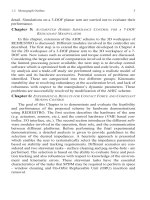
4.3 Schemes for Compliant and Force Control
of Redundant Manipulators
The problem of compliant motion control of redundant manipulators
has not attained the maturity level of its non-redundant counterpart. There
is little work that addresses the problem of redundancy resolution in a com-

pliant motion control scheme. There are two major issues to be addressed in
extending existing compliant motion schemes to the case of redundant
manipulators:
Target Trajectory
Desired T
ra
jectory
Environment
Actual T
ra
jectory
X
·
i
t
F
i
d
B
i
d

andX
·
i
t
t fo
lim
F
i

d
B
i
d

=
(i) The nature of compliant motion control requires expressing the
manipulator’s task in Cartesian space; therefore, such schemes are usually
based on the Cartesian dynamic model of manipulator. However, in the
presence of redundancy, there is not a unique map from Cartesian space to
joint space.
(ii) Most redundancy resolution techniques are at the velocity level, and
simple extensions of these techniques to the acceleration level have resulted
in the self-motion phenomenon.
For instance, Gertz et al. [23], Walker [91] and Lin et al. [39] have used
a generalized inertia-weighted inverse of the Jacobian to resolve redun-
dancy in order to reduce impact forces. However, these schemes are single
purpose algorithms, and cannot be used to satisfy additional criteria. An
extended impedance control method is discussed in [2] and [51]; the former
al
so includes an HIC scheme. These schemes can be considered as multi-
purpose algorithms since different additional tasks can be incorporated in
HIC without modifying the schemes and the control laws. However, there
ar
e
tw
o ma
jor draw
ba
cks

to
these
sc
he
mes
:
(i) The dimension of the
ad
di-
tional task should be equal to the degree of redundancy, which makes the
approach not applicable for a wide class of additional tasks, i.e., additional
tasks that are not active for
all
time such as obstacle
avoidance in a clut-
tered environment. (ii) The HIC scheme introduces the possibility of con-
trolling tasks either by a position controlled or a force controlled scheme.
The possibili
ty of having an
additional task
controlled by
a
force cont
rolled
scheme is ignored by including the additional task in the position controlled
subspace of the extended task. Shadpey et al. [72] have proposed an Aug-
ment
ed Hybrid Impedance Control (AHIC) scheme
to
overcome

these
problems (see Section 4.3.2). This scheme enjoys the following major
advantages:
(i) Different additional tasks can be easily incorporated in the AHIC
scheme without modifying the scheme and the control law.
(ii) An additional task can be included in the force-controlled subspace
of t
he augmented task. Therefore, it
is possible to have a multiple-point
force control scheme.
(iii) Task p
riority and singularity
robustness formulat
ion of th
e AHIC
scheme relaxes the restrictive assumption of having a non-singular aug-
mented Jacobian.
However, the scheme in [72] exhibits the self-motion phenomenon, i.e.,
motion of the arm in the null space of the Jacobian. Another AHIC scheme
90 4 Contact Force and Compliant Motion Control
4.3 Schemes for Compliant and Force Control of Redundant Manipulators 91
which has the above mentioned characteristics [73] is presented in Section
4.3.3. Moreover, by modifying both the inner and outer control loops, the
self-motion is damped when the dimension of the augmented task is smaller
than that of the joint space. This scheme is also more amenable to an adap-
tive implementation. An adaptive version of the AHIC scheme [74] is
described in Section 4.3.4 .
4.3.1 Configuration Control at the Acceleration Level
Similar to the pseudo-inverse solution given by (2.3.30), the following
weighted damped least-squares solution can be obtained:

(4.3.1)
This minim
izes
the following cost function:
(4.3.2)
where
(4.3.3)
However
, this solution
is
incapable of controlling
the
null
space component
of joint velocities (see Section 2.3.2 ). A remedy for this difficulty is to dif-
ferentiate the configuration control solution at the velocity level given by
equation (2.3.19). This yields
(4.3.4)
where
Therefore, following the reference joint velocity given by equation (2.3.19)
and the acceleration trajectory given by (4.3.4), we get a special solution
that minimizes the joint velocities when , i.e., there are not as many
active tasks as the degree of redundancy, and we have the best solution in
q
··
J
e
T
W
e

J
e
J
c
T
W
c
J
c
W
v
++>@
1–
J
e
T
W
e
X
··
J
·
e
q
·
–>=
J
c
T
W

c
Z
··
J
·
c
q
·
–@+
LE
··
e
T
W
e
E
··
e
E
··
c
T
W
c
E
··
c
q
··
T

W
v
q
··
++=
E
··
e
X
··
d
X
··
J
·
e
q
·
–and
E
··
c
Z
··
d
Z
··
J
·
c

q
·
––=–=
q
··
J
e
T
W
e
J
e
J
c
T
W
c
J
c
W
v
++>@
1–
AB+>@=
AJ
e
T
W
e
X

··
J
·
e
q
·
–J
c
T
W
c
Z
··
J
·
c
q
·
–+=
BJ
·
e
T
W
e
X
·
J
e
q

·
–J
·
c
T
W
c
Z
·
J
c
q
·
–+=
kr
the least-squares sense when . In all cases the presence of ensures
the boundedness of the joint velocities.
4.3.2A
ugmen
ted Hybrid Impedance
Contr
ol
using the Computed
Torque Algorithm
The AHIC scheme, shown in Figure 4.5, can be broken down into two
different control loops. The outer loop generates an Augmented Cartesian
Target Acceleration (ACTA) trajectory reflecting the desired impedancein
the position-controlled subspaces, and the desired force in the force-con-
trolled subspaces of the main and additional tasks. From this point of view,
the AHIC problem can be formulated as that of tracking an ACTA trajec-

tory which is generated in real time. The inner-loop control problem con-
sists
of selecting
an input
to the
actuators which makes the end-effector
track a desired trajectory generated by the outer loop.
Figure 4.5 Block diagram of the AHIC scheme using the computed torque
controller
4.3.2.1 Outer-loop design
The design of the outer-loop part of the AHIC scheme is described in
this section. As mentioned in Section 4.2, the idea is to split the spaces cor-
responding to the main task X and additional task Z into position- and force-
controlled subspaces. Impedance control is used in the position-controlled
subspace. Therefore, the objective is to make the manipulator act as a mass-
spring-dashpot system with desired inertia, damping, and stiffness in each
dimension of the position-controlled subspace of the main and additional
tasks. In the force-controlled subspace, a desired inertia and damping have
been introduced because, if only a simple proportional force feedback were
kr! W
v
W
ACT
generator
(additional task)
ARM
outer loop
inner loop
Des
ir

ed fo
rc
e
&
position trajectory
W
ACTA
generator
Redundancy
Resolution
(main task)
Des
ir
ed fo
rc
e
&
Desired force
&
position trajectory
Controller
Computed
torque
X
··
t
q
··
t
F

qq
·

Z
··
t
92 4 Contact Force and Compliant Motion Control
4.3
Schemes for
Compliant
and Forc
e
Contr
ol
of Redundant
Manipulators
93
applied, the response could be very under-damped for an environment with
high stiffness.
The motion
of the manipulator in both s
ubspaces
can be expressed by
a
single matrix equation using selection matrices S
x
and S
z
, as follows:
(4.3.5)

where the superscript d denotes the desired values; the subscripts x and z
refer
to
the
main and additional tasks respectively;
the diagonal matrices
M,
B, and K are the desired mass, damping, and stiffness matrices; F
d
and -F
e
are vectors of the desired and the environmental reaction forces; and S
x
and
S
z
are the diagonal selection matrices
which
ha
ve
1’
s
on the diagonal for
position-controlled subspaces and 0’s
for the force-controlled subspaces.
Solving the motion equations (4.3.5) for the accelerations and
leads to the Cartesian Target Acceleration (CTA) trajectories of the main,
,
and additional tasks,
:

(4.3.6)
Now the AHIC scheme can be formulated to track the CTA trajectories.
Using the configuration control approach - equation (4.3.1), the desired
Joint Target Acceleration (JTA) trajectory can be found by replacing
the CT
A traj
ectories of th
e main and addit
ion
al tasks in Equation
(4.3.
1).
(4.3.7)
Remark: Duffy [20] has indicated that in the case of compliant motion of a
manipulator in 3D space, the end-effector velocities (linear, angular) and
M
z
d
Z
··
S
z
Z
··
d
–B
z
d
Z
·

S
z
Z
·
d
–K
z
d
S
z
ZZ
d
–
IS
z
–F
Z
d
F
z
e
–=–
++
M
x
d
X
··
S
x

X
··
d
–B
x
d
X
·
S
x
X
·
d
–K
x
d
S
x
XX
d
–
IS
x
–F
x
d
F
x
e
–=–

++
(a)
(b)
X
··
Z
··
X
··
t
Z
··
t
X
··
t
S
x
X
··
d
M
x
d

1–
B
x
d
X

·
S
x
X
·
d
–K
x
d
S
x
XX
d
–
IS
x
–F
x
d
– F
x
+
+
>
@
–=
Z
··
t
S

z
Z
··
d
M
z
d

1–
B
z
d
Z
·
S
z
Z
·
d
–K
z
d
S
z
ZZ
d
–
IS
z
–F

Z
d
F
z
e
+–
+>
@
–=
(a)
(b)
q
··
t

q
··
t
J
e
T
W
e
J
e
J
c
T
W
c

J
c
W
v
++>@
1–
J
e
T
W
e
X
··
t
J
·
e
q
·
–
J
c
T
W
c
Z
··
t
J
·

c
q
·
–+
>
@
=
forces (forces, torques) should be considered as screws represented in axis
and ray coordinates. Therefore, in general the concept of orthogonality of
force and position controlled subspaces is not valid. As shown in [80], the
concept that is appropriate is that of “reciprocal” subspaces, i.e., the set of
motion screws should be decomposed into mutually reciprocal free and
constraint subspaces.
4.3.2.2 Inner-loop
The dynamics of a rigid manipulator in the absence of disturbances are
described by:
(4.3.8)
where is the vector of applied forces (torques), H(q) is the symmet-
ric positive definite inertia matrix, h is the vector of centrifugal and Coriolis
forces, f is the vector of frictional forces, and G is the vector of gravitational
forces. The last term on the right-hand side of the equation is only needed if
another point of the manipulator (other than the end-effector) is in contact
with the environment; denotes the reaction force corresponding to a
second constraint surface, and J
c1
is the Jacobian of the contact point.
As mentioned earlier, the responsibility of the inner loop is to ensure
that the manipulator tracks the JTA trajectory. Referring to the dynamic
equation of the manipulator, the input torque is selected by:
(4.3.9)

which guarantees perfect following of the JTA trajectory in the absence of
uncertainties in the manipulator’s parameters.
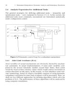
4.3.2.3 Simulation Results for a 3-DOF Planar Arm
The performance of the AHIC scheme has been studied using simula-
tions involving a 3-revolute-joint planar manipulator (Figure 4.6). In all
cases, a constraint surface is defined by the position P
c
and orientation
of a frame C attached to this surface.The main task (same for all cases),
defined in the constraint frame, is specified by a desired impedance (inertia,
damping, and stiffness) in tracking of the desired position trajectory in the
X
c
direction, and desired force trajectory in the Y
c
direction. The selected
values for the simulations are: m
d
=1, b
d
=120, and k
d
=3600. The environ-
ment is modelled as a spring with stiffness K
e
=10000 N/m. The desired
Hqq
··
hqq
·

Gq fq
·
+++ W J
e
T
F
x
e
J
c 1
T
F
z
e
++=
W nnu
F
z
e
W Hq
··
t
hqq
·
Gq fq
·
 J
e
T
F

x
e
– J
c 1
T
F
z
e
–+++=
T
c
94 4 Contact Force and Compliant Motion Control
4.3
Schemes for
Compliant
and Forc
e
Contr
ol
of Redundant
Manipulators
95
position trajectory is calculated by linear interpolation between the initial
and final points (constant velocity trajectory), and the force trajectory is
defined by f
d
= -100 N . For each individual case, a different additional task
is d
ef
ined. A

gene
ral bloc
k
dia
gram of
the
simulation is
show
n
in
Figure
4.7 where T denotes the homogenous coordinate transformation between
two different frames ( W refers to the workspace, and C refers to the end-
effector constraint surface). Note that the blocks shown by dashed lines are
needed if the only the additional task is force-controlled ( C1 refers to the
second constraint surface).
Figure
4.6
3-DOF planar mani
pul
ator used
in the simulat
ion
Joint Limit Avoidance (JLA)
The formulation of the additional task was given in Section 2.4.1 . In
the first simulation, JLA is inactive, and the resulting errors in the position
and force controlled subspaces
()
both converge
to small values

(practically
zero). However, the joint three value goes below -100 degrees. In the sec-
ond simulation, JLA is active and the minimum limit for joint three is
selected as -80
degrees. The simulatio
n results
again
show
that
the force
and position trajectories are tracked correctly, and also the limit on joint
three is respected.
Static and Moving Obstacle Avoidance (SOCA and MOCA)
The formulation of the additional task was given in Section 2.4.2 . The
results for SOCA are indicated in , When the obstacle avoidance algorithm
is inactive, the main task trajectories are followed correctly. However, a
collision occurs. By activating obstacle avoidance, the collision is avoided
and the main task requirement is also satisfied.
X
w
Y
w
X
c
Y
c
T
c
q1
q2

q3
P
c