Control of Redundant Robot Manipulators - R.V. Patel and F. Shadpey Part 9 ppt

4.3
Schemes for
Compliant
and Forc
e
Contr
ol
of Redundant
Manipulators
11
1
(4.3.16)
where are calculated based on estimated values of H, C, G,
f , and a respectively. is the measured end-effector interaction force with
the environment, is a positive-definite matrix, and . The
last term on the right-hand side of the equation is only needed if another
point of the manipulator (other than the end-effector) is in contact with the
environment; denotes the measured reaction force corresponding to a
second constraint surface, and J
c1
is the Jacobian of the contact point.
We use the same Lyapunov candidate function as in [41]:
(4.3.17)
where is a constant positive-definite matrix and . Differenti-
ating along the trajectory of the system (4.3.8) leads to
(4.3.18)
where denotes force measurement error. This suggests that
the adaptation law should be selected as:
(4.3.19)
With this adaptation law, equation (4.3.18) leads to:
(4.3.20)

an
d
(4.3.21)
where is the minimum eigenvalue value of the matrix , and satis-
fies t
he following inequality:
W Ya
ˆ
K
D
sJ–
e
T
F
ˆ
x
e
J
c 1
T
F
ˆ
z
e
––=
H
ˆ
qq
··
r

C
ˆ
qq
·
q
·
r
G
ˆ
q f
ˆ
q
·
J
e
T
– F
ˆ
x
e
J
c 1
T
F
ˆ
z
e
–++
+
=

H
ˆ
C
ˆ
G
ˆ
f
ˆ
a
ˆ

F
ˆ
x
e
K
D
sq
·
q
·
r
–=
F
z
e
Vt
1
2

s
T
Hs a
˜
T
* a
˜
+>@=
* a
˜
aa
ˆ
–=
Vt
V
·
t s
T
K
D
s– s
T
Ya
˜
s
T
J
e
T
F

˜
x
e
s
T
J
c 1
T
F
˜
z
e
++
+
=
F
˜
FF
ˆ
–=
a
ˆ
·
* Y
T
s–=
V
·
t s
T

K
D
s– s
T
J
e
T
F
˜
x
e
J
c 1
T
F
˜
z
e
+
k
D
s
2
– sJ
e
F
˜
x
e
J

c 1
F
˜
z
e
++d
+=
V
·
t k
D
s
2
– G s+d
k
D
K
D
G
(4.3.22)
We also assume that and . Now, we consider two dif-
ferent cases: precise and imprecise force measurements.
Precise force measurements
In this case, inequality (4.3.21) reduces to
(4.3.23)
which implies
or boundedness
of
a and s . Moreover
, it

can
be
shown that
(4.3.24)
which implies that and consequently . In order to
establi
sh a link between
S
and the tracking
errors of ACT trajectories, we
assume that the
tracking errors of
the damped least
-squares
solution
(2.3.19) are negligible. Therefore, multiplying both sides of equation
(4.3.13) by the augmented Jacobian, leads to
(4.3.25)
where
(4.3.26)
The equations in (4.3.25) represent strictly proper, asymptotically sta-
ble linear time-invariant systems with inputs which imply
exact tracking and asymptotic convergence of the trajectories X and Z to
the ACT trajectories [54], [59].
J
e
F
˜
x
e

J
c 1
F
˜
z
e
+ Gd
J
e
Dd J
c 1
Ed
F
˜
0=
V
·
t k
D
s
2
–d
as L
f
n

s
2
dt
1–

k
D



dV
t
d
s
2
dt
1–
k
D

dV t
0
f
³
d
0
f
³
1
k
D

V 0 V f–=
(a)
(b)

sL
2
n
 J
e
sJ
c
s L
2
n

J
e
se
·
x
/
x
e
x
+= a
J
c
se
·
z
/
z
e
z

+= b
e
x
XX
t
e
z
ZZ
t
–=–=
J
e
sJ
c
s L
2
n

112 4 Contact Force and Compliant Motion Control
4.3
Schemes for
Compliant
and Forc
e
Contr
ol
of Redundant
Manipulators
11
3

Imprecise Force Measurements (Robustness Issue)
To take into account the robustness issue, we consider the effects of
imprecise force measurements. It is obvious that error in force measure-
ments directly affects the tracking performance in the force controlled sub-
spaces of the main and additional tasks. However, we can show
boundedness of the closed-loop trajectories. Moreover, the upper-bound on
the error in the position-controlled subspaces can be reduced.
In this case, the time derivative of the Lyapunov candidate function sat-
isfies
(4.3.27)
As i
n [41], we
can
st
ate that
is
not guaranteed to
be negat
ive semi-def-
inite with an arbit
rary value of
and a lar
ge
for small values of
.
However, positive implies increasing V and subsequently , which
eventually makes negative. Therefore, s remains bounded and con-
ver
ges
to

a
residual set. For a fixed
value of
, the
lower bound on
s is
determined by and can be reduced by selecting a larger value of .
Note that larger increases the control effort and may saturate the actua-
tors. Using equations (4.3.24) and boundedness of s , we can conclude
boundedness of and .
Remark:
Dawson and Qu [17] have proposed a modification to the control
law given in (4.3.16) by adding a term to the right hand side
with . This eventually leads to the same inequality for as in
(4.3.23) which implies asymptotic convergence of the errors. However, the
control law proposed in [17] is discontinuous in terms of s and may excite
unmodeled high-frequency dynamics.
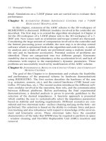
4.3.4.3 Simulation Results for a 3-DOF Planar Arm
The setup for constrained compliant motion control is shown in Figure
4.6. A general block diagram of the simulation is shown in Figure 4.14.
Tool Orientation Control
In this simulation the
additional task
is
defined as the
control
of
the ori-
entation of a tool attached to the end-effector. In this case, the desired value
F

˜
0z
V
·
t k
D
s
2
– G s+d
V
·
t
k
D
G s
V
·
t s
V
·
t
k
D
G k
D
e k
D
k
D
e

x
e
Z
K
G
ssgn–
K
G
G! V
·
t
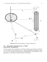
is specified as . The end-effector is initially at the point ( X=1,
Y=1) (Figures 4.17a, c) in touch with the surface (zero interaction force).
Figures 4.17a, b show that without activating the additional task, there is no
restriction on joint three. However, by activating the additional task (Fig-
ures 4.17c, d), the tool orientation is maintained at the desired value. Fig-
ures 4.18a, b show the errors in the position- and force-controlled
subspaces which practically converge to zero. The dynamic parameter esti-
mates and the velocity error are shown in Figures 4.18d, e.
Figure
4.
17
Adaptive
AHIC: Arm configuration
and joint
values
In order to study the effects of im
precise force measurements, the
actual interaction force is augmented by a random noise uniformly distrib-
uted in the interval (-15N,15N). As we can see in Figure 4.19b, the error in

the force controlled direction increases significantly as expected. The rea-
son is that the controller in the force-controlled direction is based on force
q
3
85q–=
−0.5 0 0.5 1 1.5 2
−0.5
0
0.5
1
1.5
0 0.5 1 1.5 2 2.5 3 3.5 4
−150
−100
−50
0
50
100
0 0.5 1 1.5 2 2.5 3 3.5 4
−150
−100
−50
0
50
100
150
−0.5 0 0.5 1 1.5 2
−0.5
0
0.5

1
1.5
(a
)
(b
)
(c)
(d)
q
3
q
3
a),
b) w
ith
ou
t, and
c), d)
w
it
h t
ool
orient
atio
n
co
ntro
l
Y
Y

X
X
deg
deg
114 4 Contact Force and Compliant Motion Control
4.3
Schemes for
Compliant
and Forc
e
Contr
ol
of Redundant
Manipulators
11
5
measurements and any error in this respect, directly affects the force error,
e.g., the interval between 2 to 3 seconds. However, the error in the position-
controlled direction (Figure 4.19a) remains practically unchanged from that
of the previous simulation (Figure 4.18a), showing the robustness of the
algorithm to force measurement error.
Figure 4.18 Adaptive AHIC with tool orientation control
0 0.5 1 1.5 2 2.5 3 3.5 4
−80
−70
−60
−50
−40
−30
−20

−10
0
10
20
0 0.5 1 1.5 2 2.5 3 3.5 4
−3500
−3000
−2500
−2000
−1500
−1000
−500
0
500
1000
1500
0 0.5 1 1.5 2 2.5 3 3.5 4
−15
−10
−5
0
5
10
15
20
25
30
35
0 0.5 1 1.5 2 2.5 3 3.5 4
−0.25

−0.2
−0.15
−0.1
−0.05
0
0.05
0.1
0.15
0.2
0.25
0 0.5 1 1.5 2 2.5 3 3.5 4
−0.5
0
0.5
1
1.5
2
2.5
3
x 10
−3
(c) Torques (Nm)
(d) Parameter estimates
a) Position error (m)
(e) Joint velocities (deg/s)
(b) Force error (N)
Figure 4.19 Adaptive Hybrid Impedance Control: Effect of imprecise force
measurement
4.4 Conclusions
In this chapter, the problem of compliant motion and force control for

redundant manipulators was addressed and an Augmented Hybrid Imped-
ance Control Scheme was proposed. An extension of the configuration con-
trol approach at the acceleration level was developed to perform
redundancy resolution. The most useful additional tasks: Joint limit avoid-
ance, static and moving object avoidance, and posture optimization, were
incorporated into the AHIC scheme. The proposed scheme has the follow-
ing desirable characteristics:
0 0.5 1 1.5 2 2.5 3 3.5 4
−80
−70
−60
−50
−40
−30
−20
−10
0
10
20
0 0.5 1 1.5 2 2.5 3 3.5 4
−0.5
0
0.5
1
1.5
2
2.5
3
x 10
−3

b) Force error (N)
(a) Position error (m)
116 4 Contact Force and Compliant Motion Control
4.4
Conclusio
ns
11
7
• Different additional tasks can be easily incorporated into the
AHIC scheme without modifying the scheme and the control law.
• The additional task(s) can be included in the force-controlled
subspace of the augmented task. Therefore, it is possible to have
a multiple-point force control scheme.
• Task priority and singularity robustness formulation of the AHIC
scheme relax the restrictive assumption of having a non-singular
augmented Jacobian.
A
modified AHIC scheme was proposed
in this chapter that gives a
solution to the undesirable self-motion problem which exists in most
dynamic control schemes developed for redundant manipulators. An Adap-
tive Augmented
Hybrid
Impedanc
e Control (AAHIC)
scheme was
described which guarantees asympt
otic
convergence in both
position- and

force-controlled subspaces with precise force measurements. The control
scheme also ensures stability of the system in the presence of bounded
force m
easurement errors. Even in
the
case of imprecise force
measure-
ments, the errors in the position controlled subspaces can be reduced con-
siderably. The performance of the proposed AHIC schemes was illustrated
for a
3-DOF
planar
arm. In the next
chapter,
we will
extend the AHIC
scheme to the 3-D workspace of REDIESTRO, a 7-DOF experimental
robot.
CHAPTER 5AHIC FOR A 7-DOF REDUNDANT MANIPULATOR
5.1 Introduction
In Chapter 4, the AHIC scheme was developed and verified by simula-
tion on a 3-DOF planar arm. In this chapter the extension of the AHIC
scheme to the 3-D workspace of REDIESTRO, a 7-DOF experimental
manipulator, is described. Figure 5.1 shows a simplified block diagram of
the AHIC controller. Considering that the capabilities of the redundancy
resolution scheme with respect to collision avoidance have already been
fully demonstrated, in order to focus on the new issues related to Contact
Force Control (CFC), the environment is assumed to be free of obstacles.
The complexity of the required algorithms and constraints on the
amount of computational power available have resulted in an algorithm

development procedure which incorporates a high level of optimization. At
the same time, the following issues which were not studied in the 2-D
workspace need to be tackled in extending the schemes to a 3-D workspace:
 Extension of the AHIC scheme for orientation and torque
 Control of self-motion as a result of resolving redundancy at the
acceleration level for the AHIC scheme represented in Section 4.3.2
 Robustness with respect to higher-order unmodelled dynamics
(joint flexibility), uncertainties in manipulator dynamic parameters, and
friction model.
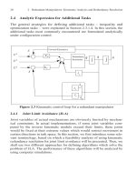
5.2 Algorithm Extension
In this section, the different modules involved in the AHIC scheme are
described. The focus is on describing the required algorithms without get-
ting involved in the specific way in which the modules are implemented.
5Augmented Hybrid Impedance Control for a
7-DOF Redundant Manipulator
R.V. Patel and F. Shadpey: Contr. of Redundant Robot Manipulators, LNCIS 316, pp. 119–145, 2005.
© Springer-Verlag Berlin Heidelberg 2005
120 5 AHIC for a 7-DOF Redundant Manipulator
Figure 5.1 Simplified block diagram of the AHIC controller
5.2.1 Task Planner and Trajectory Generator (TG)
The robot’s task can be specified using a Pre-Programmed Task File.
Each line indicates the desired position and orientation to be reached at the
end of that segment, the hybrid task specification, and the desired imped-
ance and force (if applicable) for each of the 6 DOFs.
In the absence of obstacles, the robot path will consist of straight lines
connecting the desired position/orientation at each segment. The TG mod-
ule generates a continuous path between the via points. The TG imple-
mented to test the AHIC scheme generates a fifth-order polynomial
trajectory which gives continuous position, velocity, and acceleration pro-
files with zero jerk (rate of change of acceleration) at the beginning and the

end of the motion.
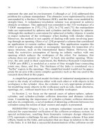
5.2.2AHIC module
Figure 5.2 shows the location of the different frames used by the AHIC
module. The description of the environment is specified in a configuration
file. As an example, for a surface-cleaning task, it is required to specify the
location and orientation of a fixed frame with respect to the world
frame. In this case, the robot’s base frame is selected as the world
frame. The tool frame is attached to the last link. Depending on the
type of the tool, the user specifies the location and orientation of this frame
AHIC
Forward
Kinematics
xx
·
,
f
d
f
f
qq
·
,
x
··
t
q
··
t
qq
·

,
qq
·
,
Traj.
Gener-
-ator
Redun-
-dancy
Resolu-
ti
on
Lineariz-
ation &
Decoupl-
in
g (Inv
.
Dyn.)
Robot &
Environ-
ment
x
d
x
·
d
x
··
d

,,
C
R
1

T
5.2
Algo
rith
m
Extension
121
in the last joint’s local frame. The force sensor interface card also uses this
information to locate the force sensor frame at . The task frame
is located at the origin of the frame . However, the orientation of
is dictated by . Therefore, the frame moves with the tool while
keeping the same orientation as the constant frame .
The AHIC scheme, as implemented for the 2-D workspace, generates
an Augmented Cartesian Target Acceleration (ACTA) for the end-effector
(EE) position in real-time:
(5.2.1)
where are diagonal matrices whose diagonal elements repre-
sent the desired mass, damping, and stiffness; S is a diagonal selection
matrix which specifies the forc
e- ()
or posi
tion- ()
con-
trolled axis; are the desired and interaction forces.
In o

rder to keep the concept
of
sp
litting
position
and
orientation
control
as described in Section 3.3.2 , the AC
TA
in the 3-D wo
rkspace wi
ll be gen-
erated separately for position/force-controlled and orientation/torque-con-
trolle
d axes
:
(5.2.2)
(5.2.3)
where the subscripts p and o indicate that
the
corresponding variables
are
specified for position/force-controlled and orientation/torque-controlled
subspaces respectively
. The superscr
ipt
d denotes the desired values. The
vector
and its derivatives are th

e
position,
velocity
,
and accelera-
tion of the origin of {T} expressed in frame {C}; and are the desired
and interaction forces expressed in {C}; is the selection matrix
T C
i

T C
i

C C
i

C
X
··
t
M
d
1–
F
e
– IS–F
d
B
d
X

·
SX
·
d
–– K
d
SX X
d
––+=
SX
··
d
+
M
d
B
d
K
d

S
i
0= S
i
1=
F
d
F
e


P
··
t
t M
p
d
1–
F
e
– IS
p
–F
d
B
p
d
P
·
S
p
P
·
d
––+=
K
P
d
S
p
PP

d
–– S
p
P
··
d
+

·
t
t M
o
d
1–
 N
e
– IS
o
–N
d
B
o
d
 S
o

d
––+=
K
o

d
S
o
e
o
–  S
o

·
d
+
P 31
F
d
F
e
S
p
33
used to indicate that a {C} frame axis is force- or position-controlled;
are the angular velocity and acceleration of the {T} frame expressed in
; is the orientation error vector (see Section 3.3.2.2 ); are
the desired and interaction torques in frame ; and are
diagonal matrices whose diagonal elements represent the desired mass,
damping, and stiffness.
Equation (5.2.2) is resolved in frame {C} while Equation (5.2.3) is
resolved in frame
. The f
ra
me

is
a time-varying
frame (in con-
trast to frame {C} which is a fixed frame) located at the origin of frame {T}
and
with same orientation as
{C}.
All the inputs and outputs in equatio
ns (5.2.2) and (5.2.3) should be
expressed in frames {C} and respectively. In order to make the AHIC
controller module self-contained, all the necessary conversions are imple-
mented in this module.
The location of the origin of {C} in () and the rota-
tion matrix
are specified in a conf
iguration file. It should be noted
that the orientations of {C} and in any arbitrary frame are the same.
5.2.3 Redundancy Resolution (RR) module
The RR module for the AHIC scheme should be implemented at the
acceleration level. Assuming an obstacle-free workspace, the
damped least-
squares solution is given by:
(5.2.4)
where

·

C
i
e

o
N
d
N
e

C
i
 M
d
B
d
K
d

C
i
 C
i

C
i

R
1
 P
R
1
C
33

R
R
1
C
C
i

q
··
t
A
1–
b=
AJ
p
T
W
p
J
p
J
o
T
W
p
J
p
J
c
T

W
c
J
c
W+
v
++=
bJ
p
T
W
p
P
··
t
J
·
p
q
·
–J
p
T
W
p

·
t
J
·

o
q
·
–J
c
T
W
c
Z
·
t
++=
122 5 AHIC for a 7-DOF Redundant Manipulator
5.2
Algo
rith
m
Extension
123
Figure 5.2 Different frames involved in the hybrid task specification
and are the Jacobian matrices projecting the joint rates to linear and
angular velocities of frame {T}. The Jacobian matrices and the two vectors
()
are calculated by the forward kinematics module. The matrices
are the diagonal weighting matrices that assign priority
between position/force tracking, orientation/torque tracking and singularity
avoidance (in the case of conflicts between these tasks), these matrices are
specified by the user in a configuration file. A complete study that demon-
strates the effects of the weighting matrices is given in Section 3.3.2.3 . The
vectors are the target linear and angular accelerations of frame {T}

expressed in the robot’s base frame. These vectors are calculated by the
AHIC module. Because the quantities are expressed in the same frame, no
coordinate transformation is needed. Note that at this stage, the additional
task that is incorporated into the system is joint limit avoidance. For the
joint limit avoidance task, the terms and reduce to
(see S
ection
2.4.1.3 ). The tar
get acceleration for
the
ith joint
in the case
of
violation of soft-joint limits is defined by:
Y
X
X
X
Z
Y
Y
Z
Z
C
i

T
C
Y
X

Z
R
1

O
T
J
p
J
o
J
·
p
q
·
J
·
o
q
·

W
p
W
o
W
v

P
··

t

·
t

J
c
T
W
c
J
c
J
c
T
W
c
W
c
(5.2.5)
where and are positive-definite proportional and derivative gain
matrices, andis the vector of maximum or minimum joint limits.
Computational considerations:
Considering the fact that the matrix A is guaranteed to be positive defi-
nite (because of the diagonal weighting matrix), a more efficient way to
solve (5.2.5) is to use the Cholesky decomposition. Equation (5.2.4) can be
written in the form
(5.2.6)
where. The Cholesky decomposition of A is given [93]
by: , where L is a lower-triangular matrix. This reduces to solving

an upper and an lower-triangular system of linear equations:
(5.2.7)
5.2.4 Forward Kinematics
This module calculates the position and orientation of frame {T}, the
linear and angular velocities of {T}, and also the Jacobian matrices relating
the linear and angular velocities of {T} to the joint rates. These quantities
are expressed in the robot’s base frame.
- Tool frame Information: It is only necessary to specify the informa-
tion to locateframe {T} in frame {7}. Therefore,
, are specified in a configuration
file which results in:
Z
·
i
t
K
v
i
q
·
i
– K
p
i
q
i
q
m
i
––=

K
p
K
v
q
m
W
v
Ax
b
=
xq
··
t
=
ALL
T
=
Ly b = L
T
xy=
Twist 
7
Length a
7
Offsetd
7

T
7

T
10
0
a
7
0 
7
cos 
7
sin– 0
0 
7
sin 
7
cos d
7

7
sin
00
01
=
124 5 AHIC for a 7-DOF Redundant Manipulator
5.2
Algo
rith
m
Extension
125
- Calculation of : Calculation of two new vectors ( )

which are required by the RR module (because of resolving redundancy at
the acceleration level) are added to the forward kinematics module. The
forward kinemati
cs function at th
e
acceleration level i
sd
efined
by:
(5.2.8)
which yields
(5.2.9)
This suggests that the following recursive algorithm, which calculates the
linear and angular accelerations of the frame {T}, can be used to calculate
the vectors ( ).
with initial values:
(5.2.10)
Note that the frames {8} and {T} are the same, and also, the frame {0} is
located at the robot’s base frame {R1}. Now, equation (5.2.9) results in:
(5.2.1
1)
J
·
p
q
·
J
·
o
q

·
 J
·
p
q
·
J
·
o
q
·

X
··
Jq
··
J
·
q
·
+=
X
··
q
··
0=
J
·
q
·

=
J
·
p
q
·
J
·
o
q
·

fori 1  n 1+=

i
i 1–
R
i
i 1–

i 1–
i 1–
=

i
i

i
i 1–
q

·
i
z
i
+=
v
·
i
i
R
i
i 1–
v
·
i 1–
i 1–

·
i 1–
i 1–
P
i 1–
i

i 1–
i 1–
++=

i 1–
i 1–

P
i 1–
i


·
i
i
R
i
i 1–

·
i 1–
i 1–

i
i 1–
q
·
i
z
i
+=

0
0
000
T
v

·
0
0
00
0

T
==
J
·
p
q
·
R
0
T
v
·
8
8
= J
·
o
q
·
R
0
T

·

8
8
=
5.2.5Linear Decoupling (Inverse Dynamics) Controller
The equation of motion of a 7-DOF manipulator, considering interaction
forces/torques with its environment, is given by
(5.2.12)
where is the symmetric positive-definite inertia matrix of the
manipulator in joint space; is the vector of centripetal and
Coriolis torques, is the gravity vector,is the
vector of interaction forces/torques exerted by the robot on the environment
at the operating point (origin of the tool frame), is the Jaco-
bian matrix relating the linear and angular velocities of the tool frame to
joint rates, is the joint friction vector, and is the
vector of applied torques at the actuators.
The torque that is required to linearize and decouple the nonlinear
equation (5.2.12) is given by:
(5.2.13)
where
(5.2.14)
and
(5.2.15)
where ^ denotes the estimated values. The optimized InvDyn function as
well as the closed-form representations of are developed in C
using the Robot Dynamics Modeling (RDM) software [78].
5.3 Testing and Verification
In the simulation developed for the purpose of verifying the integration
of the controller, the inverse dynamics and the model of the arm are
replaced by double integrators, i.e., we assume perfect knowledge of the
manipulator dynamics. However, the model of the environment is still

Mqq
··
Hqq
·
Gq fqq
·
+++  J
T
F–=
M
77
H 71
G 71 F 61
J 67
f 71  71
t
LD

1

2
+=

1
M
ˆ
qq
··
H
ˆ

qq
·
G
ˆ
q J
T
F
ˆ
+++=
InvDyn qq
·
q
··
t
F
ˆ
 =

2
f
ˆ
qq
·
=
MHG

present. The environment ismodeled by a linear spring.
126 5 AHIC for a 7-DOF Redundant Manipulator