Control of Robot Manipulators in Joint Space - R. Kelly, V. Santibanez and A. Loria Part 4 docx
Bạn đang xem bản rút gọn của tài liệu. Xem và tải ngay bản đầy đủ của tài liệu tại đây (343.86 KB, 30 trang )
72 3 Robot Dynamics
K(q,
˙
q)=
1
2
˙
q
T
M(q)
˙
q (3.15)
where M(q) is a matrix of dimension n×n referred to as the inertia matrix.
M(q) is symmetric and positive definite for all q ∈ IR
n
. The potential energy
U(q) does not have a specific form as in the case of the kinetic energy but it
is known that it depends on the vector of joint positions q.
The Lagrangian L(q,
˙
q), given by Equation (3.3), becomes in this case
L(q,
˙
q)=
1
2
˙
q
T
M(q)
˙
q −U(q) .
With this Lagrangian, the Lagrange’s equations of motion (3.4) may be
written as
d
dt
∂
∂
˙
q
1
2
˙
q
T
M(q)
˙
q
−
∂
∂q
1
2
˙
q
T
M(q)
˙
q
+
∂U(q)
∂q
= τ .
On the other hand, it holds that
∂
∂
˙
q
1
2
˙
q
T
M(q)
˙
q
= M(q)
˙
q (3.16)
d
dt
∂
∂
˙
q
1
2
˙
q
T
M(q)
˙
q
= M(q)
¨
q +
˙
M(q)
˙
q. (3.17)
Considering these expressions, the equation of motion takes the form
M(q)
¨
q +
˙
M(q)
˙
q −
1
2
∂
∂q
˙
q
T
M(q)
˙
q
+
∂U(q)
∂q
= τ ,
or, in compact form,
M(q)
¨
q + C(q,
˙
q)
˙
q + g(q)=τ (3.18)
where
C(q,
˙
q)
˙
q =
˙
M(q)
˙
q −
1
2
∂
∂q
˙
q
T
M(q)
˙
q
(3.19)
g(q)=
∂U(q)
∂q
. (3.20)
Equation (3.18) is the dynamic equation for robots of n DOF. Notice that
(3.18) is a nonlinear vectorial differential equation of the state [q
T
˙
q
T
]
T
.
C(q,
˙
q)
˙
q is a vector of dimension n called the vector of centrifugal and
Coriolis forces, g(q) is a vector of dimension n of gravitational forces or
torques and τ is a vector of dimension n called the vector of external
3.2 Dynamic Model in Compact Form 73
forces, which in general corresponds to the torques and forces applied by the
actuators at the joints.
The matrix C(q,
˙
q) ∈ IR
n×n
, called the centrifugal and Coriolis forces
matrix may be not unique, but the vector C(q,
˙
q)
˙
q is indeed unique. One way
to obtain C(q,
˙
q) is through the coefficients or so-called Christoffel symbols
of the first kind, c
ijk
(q), defined as
c
ijk
(q)=
1
2
∂M
kj
(q)
∂q
i
+
∂M
ki
(q)
∂q
j
−
∂M
ij
(q)
∂q
k
. (3.21)
Here, M
ij
(q) denotes the ijth element of the inertia matrix M(q). Indeed, the
kjth element of the matrix C(q,
˙
q), C
kj
(q,
˙
q), is given by (we do not show here
the development of the calculations to obtain such expressions, the interested
reader is invited to see the texts cited at the end of the chapter)
C
kj
(q,
˙
q)=
⎡
⎢
⎢
⎢
⎣
c
1jk
(q)
c
2jk
(q)
.
.
.
c
njk
(q)
⎤
⎥
⎥
⎥
⎦
T
˙
q . (3.22)
The model (3.18) may be viewed as a dynamic system with input, the
vector τ , and with outputs, the vectors q and
˙
q. This is illustrated in Figure
3.6.
ROBOT
✲
✲
✲
˙
Figure 3.6. Input–output representation of a robot
Each element of M(q), C(q,
˙
q) and g(q) is in general, a relatively complex
expression of the positions and velocities of all the joints, that is, of q and
˙
q.
The elements of M(q), C(q,
˙
q) and g(q) depend of course, on the geometry of
the robot in question. Notice that computation of the vector g(q) for a given
robot may be carried out with relative ease since this is given by (3.20). In
other words, the vector of gravitational torques g(q), is simply the gradient
of the potential energy function U(q).
Example 3.5. The dynamic model of the robot from Example 3.2, that
is, Equation (3.5), may be written in the generic form (3.18) by taking
M
(
q
)=
m
2
l
2
2
cos
2
(
ϕ
)
,
74 3 Robot Dynamics
C(q, ˙q)=0,
g(q)=0.
♦
Example 3.6. The Lagrangian dynamic model of the robot manipula-
tor shown in Figure 3.4 was derived in Example 3.3. A simple inspec-
tion of Equations (3.8) and (3.9) shows that the dynamic model for
this robot in compact form is
M
11
(q) M
12
(q)
M
21
(q) M
22
(q)
M(q)
¨
q +
C
11
(q,
˙
q) C
12
(q,
˙
q)
C
21
(q,
˙
q) C
22
(q,
˙
q)
C(q,
˙
q)
˙
q = τ(t)
where
M
11
(q)=
m
1
l
2
c1
+ m
2
l
2
1
+ I
1
M
12
(q)=[m
2
l
1
l
c2
cos(δ)C
21
+ m
2
l
1
l
c2
sin(δ)S
21
]
M
21
(q)=[m
2
l
1
l
c2
cos(δ)C
21
+ m
2
l
1
l
c2
sin(δ)S
21
]
M
22
(q)=[m
2
l
2
c2
+ I
2
]
C
11
(q,
˙
q)=0
C
12
(q,
˙
q)=[−m
2
l
1
l
c2
cos(δ)S
21
+ m
2
l
1
l
c2
sin(δ)C
21
]˙q
2
C
21
(q,
˙
q)=[m
2
l
1
l
c2
cos(δ)S
21
− m
2
l
1
l
c2
sin(δ)C
21
]˙q
1
C
22
(q,
˙
q)=0
That is, the gravitational forces vector is zero. ♦
The dynamic model in compact form is important because it is the model
that we use throughout the text to design controllers and to analyze the
stability, in the sense of Lyapunov, of the equilibria of the closed-loop system.
In anticipation of the material in later chapters of this text and in support of
the material of Chapter 2 it is convenient to make some remarks at this point
about the “stability of the robot system”.
In the previous examples we have seen that the model in compact form
may be rewritten in the state-space form. As a matter of fact, this property is
not limited to particular examples but stands as a fact for robot manipulators
in general. This is because the inertia matrix is positive definite and so is the
matrix M(q)
−1
; in particular, the latter always exists. This is what allows us
to express the dynamic model (3.18) of any robot of n DOF in terms of the
state vector [q
T
˙
q
T
]
T
that is, as
3.3 Dynamic Model of Robots with Friction 75
d
dt
⎡
⎣
q
˙
q
⎤
⎦
=
⎡
⎣
˙
q
M(q)
−1
[τ (t) −C(q,
˙
q)
˙
q −g(q)]
⎤
⎦
. (3.23)
Note that this constitutes a set of nonlinear differential equations of the
form (3.1). In view of this nonlinear nature, the concept of stability of a robot
in open loop must be handled with care.
We emphasize that the definition of stability in the sense of Lyapunov,
which is presented in Definition 2.2 in Chapter 2, applies to an equilibrium
(typically the origin). Hence, in studying the “stability of a robot manipula-
tor” it is indispensable to first determine the equilibria of Equation (3.23),
which describes the behavior of the robot.
The necessary and sufficient condition for the existence of equilibria of
Equation (3.23), is that τ(t) be constant (say, τ
∗
) and that there exist a
solution q
∗
∈ IR
n
to the algebraic possibly nonlinear equation, in g(q
∗
)=τ
∗
.
In such a situation, the equilibria are given by [q
T
˙
q
T
]
T
=[q
∗T
0
T
]
T
∈ IR
2n
.
In the particular case of τ ≡ 0, the possible equilibria of (3.23) are given
by [q
T
˙
q
T
]
T
=[q
∗T
0
T
]
T
where q
∗
is a solution of g(q
∗
)=0. Given the
definition of g(q) as the gradient of the potential energy U(q), we see that q
∗
corresponds to the vectors where the potential energy possesses extrema.
A particular case is that of robots whose workspace corresponds to the
horizontal plane. In this case, g(q)=0 and therefore it is necessary and
sufficient that τ (t)=0 for equilibria to exist. Indeed, the point
q
T
˙
q
T
T
=
[q
∗T
0
T
]
T
∈ IR
2n
where q
∗
is any vector of dimension n is an equilibrium.
This means that there exist an infinite number of equilibria. See also Example
2.2.
The development above makes it clear that if one wants to study the topic
of robot stability in open loop (that is, without control) one must specify the
dynamic model as well as the conditions for equilibria to exist and only then,
select one among these equilibria, whose stability is of interest. Consequently,
the question “is the robot stable? ” is ambiguous in the present context.
3.3 Dynamic Model of Robots with Friction
It is important to notice that the generic Equation (3.18) supposes that the
links are rigid, that is, they do not present any torsion or any other defor-
mation phenomena. On the other hand, we also considered that the joints
between each pair of links are stiff and frictionless. The incorporation of these
phenomena in the dynamic model of robots is presented in this and the fol-
lowing section.
Friction effects in mechanical systems are phenomena that depend on mul-
tiple factors such as the nature of the materials in contact, lubrication of the
76 3 Robot Dynamics
latter, temperature, etc. For this reason, typically only approximate models of
friction forces and torques are available. Yet, it is accepted that these forces
and torques depend on the relative velocity between the bodies in contact.
Thus, we distinguish two families of friction models: the static models, in
which the friction force or torque depends on the instantaneous relative ve-
locity between bodies and, dynamic models, which depend on the past values
of the relative velocity.
Thus, in the static models, friction is modeled by a vector f(
˙
q) ∈ IR
n
that
depends only on the joint velocity
˙
q. Friction effects are local, that is, f(
˙
q)
may be written as
f(
˙
q)=
⎡
⎢
⎢
⎢
⎢
⎢
⎣
f
1
(˙q
1
)
f
2
(˙q
2
)
.
.
.
f
n
(˙q
n
)
⎤
⎥
⎥
⎥
⎥
⎥
⎦
.
An important feature of friction forces is that they dissipate energy, that
is,
˙
q
T
f(
˙
q) > 0 ∀
˙
q = 0 ∈ IR
n
.
A “classical” static friction model is one that combines the so-called viscous
and Coulomb friction phenomena. This model establishes that the vector f (
˙
q)
is given by
f(
˙
q)=F
m1
˙
q + F
m2
sign(
˙
q) (3.24)
where F
m1
and F
m2
are n×n diagonal positive definite matrices. The elements
of the diagonal of F
m1
correspond to the viscous friction parameters while the
elements of F
m2
correspond to the Coulomb friction parameters. Furthermore,
in the model given by (3.24)
sign(
˙
q)=
⎡
⎢
⎢
⎢
⎣
sign( ˙q
1
)
sign( ˙q
2
)
.
.
.
sign( ˙q
n
)
⎤
⎥
⎥
⎥
⎦
and sign(x) is the sign “function”, given by
sign(x)=
1ifx>0
−1ifx<0.
However, sign(0) is undefined in the sense that one do not associate a partic-
ular real number to the “function” sign(x) when x =0.
In certain applications, this fact is not of much practical relevance, as for
instance, in velocity regulation, – when it is desired to maintain an operating
point involving high and medium-high constant velocity, but the definition of
3.4 Dynamic Model of Elastic-joint Robots 77
sign(0) is crucial both from theoretical and practical viewpoints, in position
control (i.e. when the control objective is to maintain a constant position).
For this reason, and in view of the fact that the “classical” model (3.24)
describes inadequately the behavior of friction at very low velocities, that is,
when bodies are at rest and start to move, this is not recommended to model
friction when dealing with the position control problem (regulation). In this
case it is advisable to use available dynamic models. The study of such models
is beyond the scope of this textbook.
Considering friction in the joints, the general dynamic equation of the
manipulator is now given by
M(q)
¨
q + C(q,
˙
q)
˙
q + g(q)+f (
˙
q)=τ . (3.25)
In general, in this text we shall not assume that friction is present in the
dynamic model unless it is explicitly mentioned. In such a case, we consider
only viscous friction.
3.4 Dynamic Model of Elastic-joint Robots
In many industrial robots, the motion produced by the actuators is transmit-
ted to the links via gears and belts. These, are not completely stiff but they
have elasticity which can be compared to that of a spring. In the case of revo-
lute joints, where the actuators are generally electric motors these phenomena
boil down to a torsion in the axis that connects the link to the rotor of the
motor. The elasticity effect in the joints is more noticeable in robots which
undergo displacements with abrupt changes in velocity. A direct consequence
of this effect, is the degradation of precision in the desired motion of the robot.
Evidently, industrial robots are designed in a way to favor the reduction of
joint elasticity, however, as mentioned above, such an effect is always present
to some degree on practically any mechanical device. An exception to this
rule is the case of the so-called direct-drive robots, in which the actuators are
directly connected to the links.
Robot dynamics and control under the consideration of joint elasticity, has
been an important topic of research since the mid-1980s and continues today.
We present below only a brief discussion.
Consider a robot manipulator composed of rigid n links connected through
revolute joints. Assume that the motion of each link is furnished by electric
motors and transmitted via a set of gears. Denote by J
i
, the moment of inertia
of the rotors about their respective rotating axes. Let r
i
be the gear reduction
ratio of each rotor; e.g. if r = 50 we say that for every 50 rotor revolutions, the
axis after the corresponding gear undergoes only one full turn. Joint elasticity
between each link and the corresponding axis after the set of gears is modeled
via a torsional spring of constant torsional ‘stiffness’, k
i
. The larger k
i
, the
78 3 Robot Dynamics
stiffer the joint. Figure 3.7 illustrates the case of a robot with two joints.
The joint positions of each link are denoted, as usual by q while the angular
positions of the axes after the set of gears are θ =[θ
1
θ
2
··· θ
n
]
T
. Due to
the elasticity, and while the robot is in motion we have, in general, q = θ.
q
2
k
2
r
2
:1
q
1
k
1
r
1
:1
τ
2
θ
2
θ
1
τ
1
Figure 3.7. Diagram of a robot with elastic joints
Typically, the position and velocity sensors are located at the level of the
rotors’ axes. Thus knowing the gears reduction rate, only θ may be determined
and in particular, q is not available. This observation is of special relevance in
control design since the variable to be controlled is precisely q, which cannot
be measured directly unless one is able to collocate appropriate sensors to
measure the links’ positions, giving a higher manufacturing cost.
Due to elasticity a given robot having n links has 2n DOF. Its generalized
coordinates are [q
T
θ
T
]
T
. The kinetic energy function of a robot with elastic
joints corresponds basically to the sum of the kinetic energies of the links and
3.4 Dynamic Model of Elastic-joint Robots 79
those of the rotors,
4
that is,
K(q,
˙
q,
˙
θ)=
1
2
˙
q
T
M(q)
˙
q +
1
2
˙
θ
T
J
˙
θ
where M(q) is the inertia matrix of the “rigid” (that is, assuming an infinite
stiffness value of k
i
for all i) robot, and J is a diagonal positive definite
matrix, whose elements are the moments of inertia of the rotors, multiplied
by the square of the gear reduction ratio, i.e.
J =
⎡
⎢
⎢
⎣
J
1
r
2
1
0 ··· 0
0 J
2
r
2
2
··· 0
.
.
.
.
.
.
.
.
.
.
.
.
00··· J
n
r
2
n
⎤
⎥
⎥
⎦
.
On the other hand, the potential energy is the sum of the gravitational
energy plus that stored in the torsional fictitious springs
5
, i.e.
U(q, θ)=U
1
(q)+
1
2
[q −θ]
T
K[q − θ] (3.26)
where U
1
(q) is the potential energy due to gravity and corresponds exactly
to that of the robot as if the joints were absolutely stiff. The matrix K is
diagonal positive definite and its elements are the ‘torsion constants’, i.e.
K =
⎡
⎢
⎢
⎣
k
1
0 ··· 0
0 k
2
··· 0
.
.
.
.
.
.
.
.
.
.
.
.
00··· k
n
⎤
⎥
⎥
⎦
.
The Lagrangian is in this case
L(q, θ,
˙
q,
˙
θ)=
1
2
˙
q
T
M(q)
˙
q +
1
2
˙
θ
T
J
˙
θ −U
1
(q) −
1
2
[q −θ]
T
K[q − θ] .
Hence, using Lagrange’s motion equations (3.4) we obtain
d
dt
⎡
⎢
⎢
⎢
⎢
⎣
∂
∂
˙
q
1
2
˙
q
T
M(q)
˙
q
∂
∂
˙
θ
1
2
˙
θ
T
J
˙
θ
⎤
⎥
⎥
⎥
⎥
⎦
−
⎡
⎢
⎢
⎢
⎢
⎣
∂
∂q
1
2
˙
q
T
M(q)
˙
q −U
1
(q) −
1
2
[q −θ]
T
K[q − θ]
∂
∂θ
−
1
2
[q −θ]
T
K[q − θ]
⎤
⎥
⎥
⎥
⎥
⎦
=
0
τ
.
4
Here, we neglect the gyroscopic and other coupling effects between the rotors and
the links.
5
We assume here that the rotors constitute uniform cylinders so that they do not
contribute to the total potential energy. Therefore, in (3.26) there is no term
‘ U
2
( )’.
80 3 Robot Dynamics
Finally, using (3.16), (3.17), (3.19) and
∂
∂θ
−
1
2
[q −θ]
T
K[q − θ]
= K[q − θ] ,
we obtain the dynamic model for elastic-joint robots as
M(q)
¨
q + C(q,
˙
q)
˙
q + g(q)+K(q −θ)=0 (3.27)
J
¨
θ −K[q − θ]=τ . (3.28)
The model above may, in turn, be written in the standard form, that is
through the state vector [q
T
θ
T
˙
q
T
˙
θ
T
]
T
as
d
dt
⎡
⎢
⎢
⎢
⎢
⎢
⎢
⎢
⎣
q
θ
˙
q
˙
θ
⎤
⎥
⎥
⎥
⎥
⎥
⎥
⎥
⎦
=
⎡
⎢
⎢
⎢
⎢
⎢
⎢
⎢
⎣
˙
q
˙
θ
M
−1
(q)[−K[q −θ] − C(q,
˙
q)
˙
q −g(q)]
J
−1
[τ + K[q −θ]]
⎤
⎥
⎥
⎥
⎥
⎥
⎥
⎥
⎦
.
Example 3.7. Consider the device shown in Figure 3.8, which consists
of one rigid link of mass m, and whose center of mass is localized
at a distance l from the rotation axis. The moment of inertia of the
link with respect to the axis that passes through its center of mass is
denoted by I. The joint is elastic and has a torsional constant k. The
rotor’s inertia is denoted by J .
The dynamic model of this device may be computed noticing that
K(˙q,
˙
θ)=
1
2
[ml
2
+ I]˙q
2
+
1
2
Jr
2
˙
θ
2
U(q,θ)=mgl[1 − cos(q)] +
1
2
k[q −θ]
2
,
which, using Lagrange’s equations (3.4), leads to
[ml
2
+ I]¨q + mgl sin(q)+k[q −θ]=0,
Jr
2
¨
θ −k[q − θ]=τ.
♦
3.4 Dynamic Model of Elastic-joint Robots 81
τ
J
r :1
θ
l
m
I,
q
k
Figure 3.8. Link with an elastic joint
Unless clearly stated otherwise, in this text we consider only robots with
stiff joints i.e. the model that we use throughout this textbook is given by
(3.18).
v
1
v
2
q
1
q
2
Figure 3.9. Example of a 2-DOF robot
82 3 Robot Dynamics
v
1
q
1
v
2
q
2
Figure 3.10. Example of a 2-DOF robot
3.5 Dynamic Model of Robots with Actuators
On a real robot manipulator the torques vector τ , is delivered by actuators
that are typically electromechanical, pneumatic or hydraulic. Such actuators
have their own dynamics, that is, the torque or force delivered is the product
of a dynamic ‘transformation’ of the input to the actuator. This input may
be a voltage or a current in the case of electromechanical actuators, fluid
(typically oil) flux or pressure in the case of hydraulic actuators. In Figures
3.9 and 3.10 we illustrate two robotic arms with 2 DOF which have actuators
transmitting the motion through gears in the first case, and through gear and
belt in the second.
Actuators with Linear Dynamics
In certain situations, some types of electromechanical actuators may be mod-
eled via second-order linear differential equations.
A common case is that of direct-current (DC) motors. The dynamic model
which relates the input voltage v applied to the motor’s armature, to the out-
put torque τ delivered by the motor, is presented in some detail in Appendix
3.5 Dynamic Model of Robots with Actuators 83
D. A simplified linear dynamic model of a DC motor with negligible armature
inductance, as shown in Figure 3.11, is given by Equation (D.16) in Appendix
D,
J
m
¨q + f
m
˙q +
K
a
K
b
R
a
˙q +
τ
r
2
=
K
a
rR
a
v (3.29)
where:
• J
m
: rotor inertia [kg m
2
],
• K
a
: motor-torque constant [N m/A],
• R
a
: armature resistance [Ω],
• K
b
: back emf [V s/rad],
• f
m
: rotor friction coefficient with respect to its hinges [N m],
• τ : net applied torque after the set of gears at the load axis [N m],
• q : angular position of the load axis [rad],
• r : gear reduction ratio (in general r 1),
• v : armature voltage [V].
Equation (3.29) relates the voltage v applied to the armature of the motor
to the torque τ applied to the load, in terms of its angular position, velocity
and acceleration.
K
a
,K
b
,R
a
v
J
m
f
m
1:r
qτ
Figure 3.11. Diagram of a DC motor
Considering that each of the n joints is driven by a DC motor we obtain
from Equation (3.29)
J
¨
q + B
˙
q + Rτ = Kv (3.30)
with
J = diag {J
m
i
}
B = diag
f
m
i
+
K
a
K
b
R
a
i
84 3 Robot Dynamics
R = diag
1
r
2
i
(3.31)
K = diag
K
a
R
a
i
1
r
i
where for each motor (i =1, ···,n), J
m
i
corresponds to the rotor inertia, f
m
i
to the damping coefficient, (K
a
K
b
/R
a
)
i
to an electromechanical constant and
r
i
to the gear reduction ratio.
Thus, the complete dynamic model of a manipulator (considering friction
in the joints) and having its actuators located at the joints
6
is obtained by
substituting τ from (3.30) in (3.25),
(RM(q)+J)
¨
q + RC(q,
˙
q)
˙
q + R g(q)+R f (
˙
q)+B
˙
q = Kv . (3.32)
The equation above may be considered as a dynamic system whose input
is v and whose outputs are q and
˙
q. A block-diagram for the model of the
manipulator with actuators, given by (3.32), is depicted in Figure 3.12.
˙
q
q
τ
v
¨
q
ACTUATORS
ROBOT
Figure 3.12. Block-diagram of a robot with its actuators
Example 3.8. Consider the pendulum depicted in Figure 3.13. The de-
vice consists of a DC motor coupled mechanically through a set of
gears, to a pendular arm moving on a vertical plane under the action
of gravity.
The equation of motion for this device including its load is given
by
J + ml
2
¨q + f
L
˙q +[m
b
l
b
+ ml] g sin(q)=τ
where:
• J : arm inertia without load (i.e. with m = 0), with respect to the
axis of rotation;
• m
b
: arm mass (without load);
6
Again, we neglect the gyroscopic and other coupling effects between the rotors
and the links.
3.5 Dynamic Model of Robots with Actuators 85
v
K
a
,K
b
,R
a
J
m
f
m
1:r
f
L
l
b
l
m
b
,J
m
q
Figure 3.13. Pendular device with a DC motor
• l
b
: distance from the rotating axis to the arm center of mass
(without load);
• m : load mass at the tip of the arm (assumed to be punctual
7
);
• l : distance from the rotating axis to the load m;
• g : gravity acceleration;
• τ : applied torque at the rotating axis;
• f
L
: friction coefficient of the arm and its load.
The equation above may also be written in the compact form
J
L
¨q + f
L
˙q + k
L
sin(q)=τ
where
J
L
= J + ml
2
k
L
=[m
b
l
b
+ ml]g.
Hence, the complete dynamic model of the pendular device may
be obtained by substituting τ from the model of the DC motor, (3.29),
in the equation of the pendular arm, i.e.
J
m
+
J
L
r
2
¨q +
f
m
+
f
L
r
2
+
K
a
K
b
R
a
˙q +
k
L
r
2
sin(q)=
K
a
rR
a
v,
from which, by simple inspection, comparing to (3.32), we identify
7
That is, it is all concentrated at a point – the center of mass – and has no “size”
or shape.
86 3 Robot Dynamics
M(q)=J
L
R =
1
r
2
B = f
m
+
K
a
K
b
R
a
C(q, ˙q)=0
J = J
m
K =
K
a
rR
a
f(˙q)=f
L
˙q
g(q)=k
L
sin(q) .
♦
The robot-with-actuators Equation (3.32) may be simplified considerably
when the gear ratios r
i
are sufficiently large. In such case (r
i
1), we have
R ≈ 0 and Equation (3.32) may be approximated by
J
¨
q + B
˙
q ≈ Kv .
That is, the nonlinear dynamics (3.25) of the robot may be neglected. This can
be explained in the following way. If the gear reduction ratio is large enough,
then the associated dynamics of the robot-with-actuators is described only
by the dynamics of the actuators. This is the main argument that supports
the idea that a good controller for the actuators is also appropriate to control
robots having such actuators and geared transmissions with a high reduction
ratio.
It is important to remark that the parameters involved in Equation (3.30)
depend exclusively on the actuators, and not on the manipulator nor on its
load. Therefore, it is reasonable to assume that such parameters are constant
and known.
Since the gear ratio r
i
is assumed to be nonzero, the matrix R given by
(3.31) is nonsingular and therefore, R
−1
exists and Equation (3.32) may be
rewritten as
M
(q)
¨
q + C(q,
˙
q)
˙
q + g(q)+f (
˙
q)+R
−1
B
˙
q = R
−1
Kv (3.33)
where M
(q)=M(q)+R
−1
J .
The existence of the matrix M
(q)
−1
allows us to express the model (3.33)
in terms of the state vector [q
˙
q]as
d
dt
⎡
⎣
q
˙
q
⎤
⎦
=
⎡
⎣
˙
q
M
(q)
−1
R
−1
Kv − R
−1
B
˙
q −C(q,
˙
q)
˙
q −g(q) − f (
˙
q)
⎤
⎦
.
That is, the input torque becomes simply a voltage scaled by R
−1
K.At
this point and in view of the scope of this textbook we may already formulate
the problem of motion control for the system above, under the conditions
3.5 Dynamic Model of Robots with Actuators 87
previously stated. Given a set of bounded vectors q
d
,
˙
q
d
and
¨
q
d
, determine a
vector of voltages v, to be applied to the motors, in such a manner that the
positions q, associated to the joint positions of the robot, follow precisely q
d
.
This is the main subject of study in the succeeding chapters.
Actuators with Nonlinear Dynamics
A dynamic model that characterizes a wide variety of actuators is described
by the equations
˙
x = m(q,
˙
q, x)+G(q,
˙
q, x)u (3.34)
τ = l(q, x) (3.35)
where u ∈ IR
n
and x ∈ IR
n
are the input vectors and the state variables
corresponding to the actuator and m, G and l are nonlinear functions. In
the case of DC motors, the input vector u, represents the vector of voltages
applied to each of the n motors. The state vector x represents, for instance,
the armature current in a DC motor or the operating pressure in a hydraulic
actuator. Since the torques τ are, generally speaking, delivered by different
kinds of actuators, the vector m(q,
˙
q, x) and the matrix G(q,
˙
q, x) are such
that the ∂l(q, x)/∂x
T
and G(q,
˙
q, x) are diagonal nonsingular matrices.
For the sake of illustration, consider the model of a DC motor with a non-
negligible armature inductance (L
a
≈ 0) as described in Appendix D, that
is,
v = L
a
di
a
dt
+ R
a
i
a
+ K
b
r ˙q
τ = rK
a
i
a
where v is the input (armature voltage), i
a
is the direct armature current and
τ is the torque applied to the load, after the set of gears. The rest of the
constants are defined in Appendix D. These equations may be written in the
generic form (3.34) and (3.35),
d
x
i
a
dt
=
m(q, ˙q,x)
−L
−1
a
[R
a
i
a
+ K
b
r ˙q]+
G(q, ˙q,x)
L
−1
a
u
v
τ = rK
a
i
a
l(q, x)
.
Considering that the actuators’ models are given by (3.34) and (3.35), the
model of the robot with such actuators may be written in terms of the state
vector [q
˙
qx], as
88 3 Robot Dynamics
d
dt
⎡
⎢
⎢
⎢
⎣
q
˙
q
x
⎤
⎥
⎥
⎥
⎦
=
⎡
⎢
⎢
⎢
⎣
˙
q
M(q)
−1
[l(q, x) − C(q,
˙
q)
˙
q −g(q)]
m(q,
˙
q, x)
⎤
⎥
⎥
⎥
⎦
+
⎡
⎢
⎢
⎢
⎣
0
0
G(q,
˙
q, x)
⎤
⎥
⎥
⎥
⎦
u .
The dynamics of the actuators must be taken into account in the model
of a robot, whenever these dynamics are not negligible with respect to that of
the robot. Specifically for robots which are intended to perform high precision
tasks.
Bibliography
Further facts and detailed developments on the kinematic and dynamic models
of robot manipulators may be consulted in the following texts:
• Paul R., 1982, “Robot manipulators: Mathematics, programming and con-
trol”, The MIT Press, Cambridge, MA.
• Asada H., Slotine J. J., 1986, “Robot analysis and control”, Wiley, New
York.
• Fu K., Gonzalez R., Lee C., 1987, “Robotics: control, sensing, vision, and
intelligence”, McGraw-Hill.
• Craig J., 1989, “Introduction to robotics: Mechanics and control”, Addison-
Wesley, Reading, MA.
• Spong M., Vidyasagar M., 1989, “Robot dynamics and control”, Wiley,
New York.
• Yoshikawa T., 1990, “Foundations of robotics: Analysis and control”, The
MIT Press.
The method of assigning the axis z
i
as the rotation axis of the ith joint
(for revolute joints) or as an axis parallel to the axis of translation at the ith
joint (for prismatic joints) is taken from
• Craig J., 1989, “Introduction to robotics: Mechanics and control”, Addison-
Wesley, Reading, MA.
• Yoshikawa T., 1990, “Foundations of robotics: Analysis and control”, The
MIT Press.
It is worth mentioning that the notation above does not correspond to that of
the so-called Denavit–Hartenberg convention, which may be familiar to some
readers, but it is intuitively simpler and has several advantages.
Solution techniques to the inverse kinematics problem are detailed in
Bibliography 89
• Chiaverini S., Siciliano B., Egeland O., 1994, “Review of the damped least–
square inverse kinematics with experiments on a industrial robot manipu-
lator”, IEEE Transactions on Control Systems Technology, Vol. 2, No. 2,
June, pp. 123–134.
• Mayorga R. V., Wong A. K., Milano N., 1992, “A fast procedure for ma-
nipulator inverse kinematics evaluation and pseudo-inverse robustness”,
IEEE Transactions on Systems, Man, and Cybernetics, Vol. 22, No. 4,
July/August, pp. 790–798.
Lagrange’s equations of motion are presented in some detail in the above-
cited texts and also in
• Hauser W., 1966, “Introduction to the principles of mechanics”, Addison-
Wesley, Reading MA.
• Goldstein H., 1974, “Classical mechanics”, Addison-Wesley, Reading MA.
A particularly simple derivation of the dynamic equations for n-DOF
robots via Lagrange’s equations is presented in the text by Spong and
Vidyasagar (1989) previously cited.
The derivation of the dynamic model of elastic-joint robots may also be
studied in the text by Spong and Vidyasagar (1989) and in
• Burkov I. V., Zaremba A. T., 1987, “Dynamics of elastic manipulators with
electric drives”, Izv. Akad. Nauk SSSR Mekh. Tverd. Tela, Vol. 22, No. 1,
pp. 57–64. English translation in Mechanics of Solids, Allerton Press.
• Marino R., Nicosia S., 1985, “On the feedback control of industrial robots
with elastic joints: a singular perturbation approach”, 1st IFAC Symp.
Robot Control, pp. 11–16, Barcelona, Spain.
• Spong M., 1987, “Modeling and control of elastic joint robots”, ASME
Journal of Dynamic Systems, Measurement and Control, Vol. 109, De-
cember.
The topic of electromechanical actuator modeling and its consideration in
the dynamics of manipulators is treated in the text by Spong and Vidyasagar
(1989) and also in
• Luh J., 1983, “Conventional controller design for industrial robots–A tuto-
rial”, IEEE Transactions on Systems, Man and Cybernetics, Vol. SMC-13,
No. 3, June, pp. 298–316.
• Tourassis V., 1988, “Principles and design of model-based robot con-
trollers”, International Journal of Control, Vol. 47, No. 5, pp. 1267–1275.
• Yoshikawa T., 1990, “Foundations of robotics. Analysis and control”, The
MIT Press.
90 3 Robot Dynamics
• Tarn T. J., Bejczy A. K., Yun X., Li Z., 1991, “Effect of motor dynamics
on nonlinear feedback robot arm control”, IEEE Transactions on Robotics
and Automation, Vol. 7, No. 1, February, pp. 114–122.
Problems
1. Consider the mechanical device analyzed in Example 3.2. Assume now
that this device has friction on the axis of rotation, which is modeled here
as a torque or force proportional to the velocity (f>0 is the friction
coefficient). The dynamic model in this case is
m
2
l
2
2
cos
2
(ϕ)¨q + f ˙q = τ.
Rewrite the model in the form
˙
x = f(t, x) with x =[q ˙q]
T
.
a) Determine the conditions on the applied torque τ for the existence of
equilibrium points.
b) Considering the condition on τ of the previous item, show by using
Theorem 2.2 (see page 44), that the origin [q ˙q]
T
=[0 0]
T
is a stable
equilibrium.
Hint: Use the following Lyapunov function candidate
V (q, ˙q)=
1
2
q +
m
2
l
2
2
cos
2
(ϕ)
f
˙q
2
+
1
2
˙q
2
.
2. Consider the mechanical device depicted in Figure 3.14.
A simplistic model of such a device is
m¨q + f ˙q + kq + mg = τ, q(0), ˙q(0) ∈ IR
where
• m>0 is the mass
• f>0 is the friction coefficient
• k>0 is the stiffness coefficient of the spring
• g is the acceleration of gravity
• τ is the applied force
• q is the vertical position of the mass m with respect to origin of the
plane x–y.
Write the model in the form
˙
x = f(t, x) where x =[q ˙q]
T
.
a) What restrictions must be imposed on τ so that there exist equilibria?
b) Is it possible to determine τ so that the only equilibrium is the origin,
x = 0 ∈ IR
2
?
Problems 91
y
x
k
q
f
m
Figure 3.14. Problem 2
l
1
x
0
z
0
y
0
q
1
m
1
z
o2
y
0
l
2
m
2
q
1
q
2
q
2
x
0
z
0
y
o2
Figure 3.15. Problems 3 and 4
3. Consider the mechanical arm shown in Figure 3.15.
Assume that the potential energy U(q
1
,q
2
) is zero when q
1
= q
2
=0.
Determine the vector of gravitational torques g(q),
g(q)=
g
1
(q
1
,q
2
)
g
2
(q
1
,q
2
)
.
4. Consider again this mechanical device but with its simplified description
as depicted in Figure 3.15.
a) Obtain the direct kinematics model of the device, i.e. determine the
relations
y
02
= f
1
(q
1
,q
2
)
z
02
= f
2
(q
1
,q
2
) .
92 3 Robot Dynamics
b) The analytical Jacobian J(q) of a robot is the matrix
J(q)=
∂
∂q
ϕ(q)=
⎡
⎢
⎢
⎢
⎢
⎢
⎢
⎢
⎢
⎢
⎢
⎣
∂
∂q
1
ϕ
1
(q)
∂
∂q
2
ϕ
1
(q) ···
∂
∂q
n
ϕ
1
(q)
∂
∂q
1
ϕ
2
(q)
∂
∂q
2
ϕ
2
(q) ···
∂
∂q
n
ϕ
2
(q)
.
.
.
.
.
.
.
.
.
.
.
.
∂
∂q
1
ϕ
m
(q)
∂
∂q
2
ϕ
m
(q) ···
∂
∂q
n
ϕ
m
(q)
⎤
⎥
⎥
⎥
⎥
⎥
⎥
⎥
⎥
⎥
⎥
⎦
where ϕ(q) is the relation in the direct kinematics model (x = ϕ(q)),
n is the dimension of q and m is the dimension of x. Determine the
Jacobian.
5. Consider the 2-DOF robot shown in Figure 3.16, for which the meaning
of the constants and variables involved is as follows:
τ
2
δ
q
2
l
1
l
c1
q
1
I
1
,m
1
m
2
y
z
x
τ
1
Figure 3.16. Problem 5
• m
1
,m
2
are the masses of links 1 and 2 respectively;
• I
1
is the moment of inertia of link 1 with respect to the axis parallel
to the axis x which passes through its center of mass; the moment of
inertia of the second link is supposed negligible;
• l
1
is the length of link 1;
• l
c1
is the distance to the center of mass of link 1 taken from its rotation
axis;
• q
1
is the angular position of link 1 measured with respect to the hori-
zontal (taken positive counterclockwise);
Problems 93
• q
2
is the linear position of the center of mass of link 2 measured from
the edge of link 1;
• δ is negligible (δ = 0).
Determine the dynamic model and write it in the form
˙
x = f(t, x) where
x =[q ˙q]
T
.
6. Consider the 2-DOF robot depicted in Figure 3.17. Such a robot has a
transmission composed of a set of bar linkage at its second joint. Assume
that the mass of the lever of length l
4
associated with actuator 2 is negli-
gible.
l
1
l
c2
I
3
l
4
I
2
,m
2
q
2
q
1
l
1
l
4
z
y
l
c1
I
1
,m
1
l
c3
x
m
3
link 1
actuator 1
actuator 2
link 1
Figure 3.17. Problem 6
Determine the dynamic model. Specifically, obtain the inertia matrix
M(q) and the centrifugal and Coriolis matrix C(q,
˙
q).
Hint: See the robot presented in Example 3.3. Both robots happen to be
mechanically equivalent when taking m
3
= I
3
= δ =0.
4
Properties of the Dynamic Model
In this chapter we present some simple but fundamental properties of the
dynamic model for n-DOF robots given by Equation (3.18), i.e.
M(q)
¨
q + C(q,
˙
q)
˙
q + g(q)=τ . (4.1)
In spite of the complexity of the dynamic Equation (4.1), which describes
the behavior of robot manipulators, this equation and the terms which consti-
tute it have properties that are interesting in themselves for control purposes.
Besides, such properties are of particular importance in the study of control
systems for robot manipulators. Only properties that are relevant to control
design and stability analysis via Lyapunov’s direct method (see Section 2.3.4
in Chapter 2) are presented. The reader is invited to see the references at the
end of the chapter to prove further.
These properties, which we use extensively in the sequel, may be classified
as follows:
• properties of the inertia matrix M(q);
• properties of the centrifugal and Coriolis forces matrix C(q,
˙
q);
• properties of the gravitational forces and torques vector g(q);
• properties of the residual dynamics.
Each of these items is treated independently and constitute the material of
this chapter. Some of the proofs of the properties that are established below
may be consulted in the references which are listed at the end of the chapter
and others are developed in Appendix C.
4.1 The Inertia Matrix
The inertia matrix M (q) plays an important role both in the robot’s dynamic
model as well as in control design. The properties of the inertia matrix which is
96 4 Properties of the Dynamic Model
closely related to the kinetic energy function K =
1
2
˙
q
T
M(q)
˙
q, are exhaustively
used in control design for robots. Among such properties we underline the
following.
Property 4.1. Inertia matrix M(q)
The inertia matrix M(q) is symmetric positive definite and has dimension
n ×n. Its elements are functions only of q. The inertia matrix M(q) satisfies
the following properties.
1.
There exists a real positive number α such that
M(q) ≥ αI ∀ q ∈ IR
n
where I denotes the identity matrix of dimension n×n. The matrix
M(q)
−1
exists and is positive definite.
2.
For robots having only revolute joints there exists a constant β>0
such that
λ
Max
{M(q)}≤β ∀ q ∈ IR
n
.
One way of computing β is
β ≥ n
max
i,j,q
|M
ij
(q)|
where M
ij
(q) stands for the ijth element of the matrix M(q).
3.
For robots having only revolute joints there exists a constant k
M
>
0 such that
M(x)z −M(y)z≤k
M
x − yz (4.2)
for all vectors x, y, z ∈ IR
n
. One simple way to determine k
M
is
as follows
k
M
≥ n
2
max
i,j,k,q
∂M
ij
(q)
∂q
k
. (4.3)
4.
For robots having only revolute joints there exists a number k
M
>
0 such that
M(x)y≤k
M
y
for all x, y ∈ IR
n
.
The reader interested in the proof of Inequality (4.2) is invited to see
Appendix C.
4.2 The Centrifugal and Coriolis Forces Matrix 97
An obvious consequence of Property 4.1 and, in particular of the fact that
M(q) is positive definite, is that the function V :IR
n
×IR
n
→ IR
+
, defined as
V (q,
˙
q)=
˙
q
T
M(q)
˙
q
is positive definite in
˙
q. As a matter of fact, notice that with the previous
definition we have V (q,
˙
q)=2K(q,
˙
q) where K(q,
˙
q) corresponds to the kinetic
energy function of the robot, (3.15).
4.2 The Centrifugal and Coriolis Forces Matrix
The properties of the Centrifugal and Coriolis matrix C(q,
˙
q) are important
in the study of stability of control systems for robots. The main properties of
such a matrix are presented below.
Property 4.2. Coriolis matrix C(q,
˙
q)
The centrifugal and Coriolis forces matrix C(q,
˙
q) has dimension n×n and its
elements are functions of q and
˙
q. The matrix C(q,
˙
q) satisfies the following.
1.
For a given manipulator, the matrix C(q,
˙
q) may not be unique
but the vector C(q,
˙
q)
˙
q is unique.
2.
C(q, 0) = 0 for all vectors q ∈ IR
n
.
3.
For all vectors q, x, y, z ∈ IR
n
and any scalar α we have
C(q, x)y = C(q, y)x
C(q, z + αx)y = C(q, z)y + αC(q, x)y .
4.
The vector C(q, x)y may be written in the form
C(q, x)y =
⎡
⎢
⎢
⎢
⎢
⎢
⎣
x
T
C
1
(q)y
x
T
C
2
(q)y
.
.
.
x
T
C
n
(q)y
⎤
⎥
⎥
⎥
⎥
⎥
⎦
(4.4)
where C
k
(q) are symmetric matrices of dimension n × n for all
k =1, 2, ···,n. The ij-th element C
k
ij
(q) of the matrix C
k
(q)
corresponds to the so-called Christoffel symbol of the first kind
c
jik
(q) and which is defined in (3.21).