Control of Robot Manipulators in Joint Space - R. Kelly, V. Santibanez and A. Loria Part 10 pps
Bạn đang xem bản rút gọn của tài liệu. Xem và tải ngay bản đầy đủ của tài liệu tại đây (371.51 KB, 30 trang )
Bibliography 259
• For any selection of the symmetric positive definite matrices K
p
and K
v
,
the origin of the closed-loop equation of robots with the PD control law
with compensation, expressed in terms of the state vector
˜
q
T
˙
˜
q
T
T
,is
globally uniformly asymptotically stable. Therefore, the PD control law
with compensation satisfies the motion control objective, globally. This
implies in particular, that for any initial position error
˜
q(0) ∈ IR
n
and any
velocity error
˙
˜
q(0) ∈ IR
n
,wehavelim
t→∞
˜
q(t)=0.
• For any choice of the symmetric positive definite matrices K
p
and K
v
, the
origin of the closed-loop equation of a robot with the PD+ control law,
expressed in terms of the state vector
˜
q
T
˙
˜
q
T
T
, is globally uniformly
asymptotically stable. Therefore, PD+ control satisfies the motion control
objective, globally. In particular, for any initial position error
˜
q(0) ∈ IR
n
and velocity error
˙
˜
q(0) ∈ IR
n
, we have lim
t→∞
˜
q(t)=0.
Bibliography
The structure of the PD control law with compensation has been proposed
and studied in
• Slotine J. J., Li W., 1987. “On the adaptive control of robot manipulators”,
The International Journal of Robotics Research, Vol. 6, No. 3, pp. 49–59.
• Slotine J. J., Li W., 1988. “Adaptive manipulator control: A case study”,
IEEE Transactions on Automatic Control, Vol. AC-33, No. 11, November,
pp. 995–1003.
• Slotine J. J., Li W., 1991, “Applied nonlinear control”, Prentice-Hall.
The Lyapunov function (11.3) for the analysis of global uniform asymptotic
stability for the PD control law with compensation was proposed in
• Spong M., Ortega R., Kelly R., 1990, “Comments on “Adaptive manip-
ulator control: A case study”, IEEE Transactions on Automatic Control,
Vol. 35, No. 6, June, pp.761–762.
• Egeland O., Godhavn J. M., 1994, “A note on Lyapunov stability for an
adaptive robot controller”, IEEE Transactions on Automatic Control, Vol.
39, No. 8, August, pp. 1671–1673.
The structure of the PD+ control law was proposed in
• Koditschek D. E., 1984, “Natural motion for robot arms”, Proceedings
of the IEEE 23th Conference on Decision and Control, Las Vegas, NV.,
December, pp. 733–735.
260 11 PD+ Control and PD Control with Compensation
PD+ control was originally presented in
2
• Paden B., Panja R., 1988, “Globally asymptotically stable PD+ controller
for robot manipulators”, International Journal of Control, Vol. 47, No. 6,
pp. 1697–1712.
The material in Subsection 11.2.1 on the Lyapunov function to show global
uniform asymptotic stability is taken from
• Whitcomb L. L., Rizzi A., Koditschek D. E., 1993, “Comparative experi-
ments with a new adaptive controller for robot arms”, IEEE Transactions
on Robotics and Automation, Vol. 9, No. 1, February, pp. 59–70.
Problems
1. Consider the model of an ideal pendulum studied in Example 2.2 (see
page 30)
J ¨q + mgl sin(q)=τ.
Assume that we apply the PD controller with compensation
τ = k
p
˜q + k
v
˙
˜q + J[¨q
d
+ λ
˙
˜q]+mgl sin(q)
where λ = k
p
/k
v
, k
p
and k
v
are positive numbers.
a) Obtain the closed-loop equation in terms of the state vector
˜q
˙
˜q
T
.
Verify that the origin is its unique equilibrium point.
b) Show that the origin
˜q
˙
˜q
T
= 0 ∈ IR
2
is globally asymptotically
stable .
Hint: Use the Lyapunov function candidate
V (˜q,
˙
˜q)=
1
2
J
˙
˜q + λ˜q
2
+ k
p
˜q
2
.
2. Consider PD+ control for the ideal pendulum presented in Example 11.2.
Propose a Lyapunov function candidate to show that the origin
˜q
˙
˜q
=
[0 0]
T
= 0 ∈ IR
2
of the closed-loop equation
ml
2
¨
˜q + k
v
˙
˜q + k
p
˜q =0
is a globally asymptotically stable equilibrium point.
2
This, together with PD control with compensation were the first controls with
rigorous proofs of global uniform asymptotic stability proposed for the motion
control problem.
Problems 261
3. Consider the model of the pendulum from Example 3.8 and illustrated in
Figure 3.13,
J
m
+
J
L
r
2
¨q +
f
m
+
f
L
r
2
+
K
a
K
b
R
a
˙q +
k
L
r
2
sin(q)=
K
a
rR
a
v
where
• v is the armature voltage (input)
• q is the angular position of the pendulum with respect to the vertical
(output),
and the rest of the parameters are constants related to the electrical and
mechanical parts of the system and which are positive and known.
It is desired to drive the angular position q(t) to a constant value q
d
.For
this, we propose to use the following control law of type PD+
3
,
v =
rR
a
K
a
k
p
˜q −k
v
˙q +
k
L
r
2
sin(q)
with k
p
and k
v
positive design constants and ˜q(t)=q
d
− q(t).
a) Obtain the closed-loop equation in terms of the state [˜q ˙q]
T
.
b) Verify that the origin is an equilibrium and propose a Lyapunov func-
tion to demonstrate its stability.
c) Could it be possible to show as well that the origin is actually globally
asymptotically stable?
4. Consider the control law
τ = K
p
˜
q + K
v
˙
˜
q + M(q)
¨
q
d
+ C(q,
˙
q
d
)
˙
q + g(q) .
a) Point out the difference with respect to the PD+ control law given by
Equation (11.7)
b) Show that in reality, the previous controller is equivalent to the PD+
controller.
Hint: Use Property 4.2.
5. Verify Equation (11.6) by use of (11.5) .
3
Notice that since the task here is position control, in this case the controller is
simply of type PD with gravity compensation.
12
Feedforward Control and PD Control plus
Feedforward
The practical implementation of controllers for robot manipulators is typically
carried out using digital technology. The way these control systems operate
consists basically of the following stages:
• sampling of the joint position q (and of the velocity
˙
q);
• computation of the control action τ from the control law;
• the ‘order’ to apply this control action is sent to the actuators.
In certain applications where it is required that the robot realize repetitive
tasks at high velocity, the previous stages must be executed at a high cadence.
The bottleneck in time-consumption terms, is the computation of the control
action τ . Naturally, a reduction in the time for computation of τ has the ad-
vantage of a higher processing frequency and hence a larger potential for the
execution of ‘fast’ tasks. This is the main reason for the interest in controllers
that require “little” computing power. In particular, this is the case for con-
trollers that use information based on the desired positions, velocities, and
accelerations q
d
(t),
˙
q
d
(t), and
¨
q
d
(t) respectively. Indeed, in repetitive tasks
the desired position q
d
(t) and its time derivatives happen to be vectorial pe-
riodic functions of time and moreover they are known once the task has been
specified. Once the processing frequency has been established, the terms in
the control law that depend exclusively on the form of these functions, may
be computed and stored in memory, in a look-up table. During computation
of the control action, these precomputed terms are simply collected out of
memory, thereby reducing the computational burden.
In this chapter we consider two control strategies which have been sug-
gested in the literature and which make wide use of precomputed terms in
their respective control laws:
• feedforward control;
• PD control plus feedforward.
Each of these controllers is the subject of a section in the present chapter.
264 12 Feedforward Control and PD Control plus Feedforward
12.1 Feedforward Control
Among the conceptually simplest control strategies that may be used to con-
trol a dynamic system we find the so-called open-loop control, where the
controller is simply the inverse dynamics model of the system evaluated along
the desired reference trajectories.
For the case of linear dynamic systems, this control technique may be
roughly sketched as follows. Consider the linear system described by
˙
x = Ax + u
where x ∈ IR
n
is the state vector and at same time the output of the system,
A ∈ IR
n×n
is a matrix whose eigenvalues λ
i
{A} have negative real part,
and u ∈ IR
n
is the input to the system. Assume that we specify a vectorial
function x
d
as well as its time derivative
˙
x
d
to be bounded. The control goal
is that x(t) → x
d
(t) when t →∞. In other words, defining the errors vector
˜
x = x
d
−x, the control problem consists in designing a controller that allows
one to determine the input u to the system so that lim
t→∞
˜
x(t)=0. The
solution to this control problem using the inverse dynamic model approach
consists basically in substituting x and
˙
x with x
d
and
˙
x
d
in the equation of
the system to control, and then solving for u, i.e.
u =
˙
x
d
− Ax
d
.
In this manner, the system formed by the linear system to control and the
previous controller satisfies
˙
˜
x = A
˜
x
which in turn is a linear system of the new state vector
˜
x and moreover we
know from linear systems theory that since the eigenvalues of the matrix A
have negative real parts, then lim
t→∞
˜
x(t)=0 for all
˜
x(0) ∈ IR
n
.
In robot control, this strategy provides the supporting arguments to the
following argument. If we apply a torque τ at the input of the robot, the
behavior of its outputs q and
˙
q is governed by (III.1), i.e.
d
dt
⎡
⎣
q
˙
q
⎤
⎦
=
⎡
⎣
˙
q
M(q)
−1
[τ − C(q,
˙
q)
˙
q − g(q)]
⎤
⎦
. (12.1)
If we wish that the behavior of the outputs q and
˙
q be equal to that
specified by q
d
and
˙
q
d
respectively, it seems reasonable to replace q,
˙
q and
¨
q
by q
d
,
˙
q
d
, and
¨
q
d
in the Equation (12.1) and to solve for τ . This reasoning
leads to the equation of the feedforward controller, given by
τ = M(q
d
)
¨
q
d
+ C(q
d
,
˙
q
d
)
˙
q
d
+ g(q
d
) . (12.2)
12.1 Feedforward Control 265
Notice that the control action τ does not depend on q nor on
˙
q, that is,
it is an open loop control. Moreover, such a controller does not possess any
design parameter. As with any other open-loop control strategy, this approach
needs the precise knowledge of the dynamic system to be controlled, that is,
of the dynamic model of the manipulator and specifically, of the structure
of the matrices M(q), C(q,
˙
q) and of the vector g(q) as well as knowledge
of their parameters (masses, inertias etc.). For this reason it is said that the
feedforward control is (robot-) ‘model-based’. The interest in a controller of
this type resides in the advantages that it offers in implementation. Indeed,
having determined q
d
,
˙
q
d
and
¨
q
d
(in particular for repetitive tasks), one may
determine the terms M(q
d
), C(q
d
,
˙
q
d
) and g(q
d
) off-line and easily compute
the control action τ according to Equation (12.2). This motivates the qualifier
“feedforward” in the name of this controller.
Nonetheless, one should not forget that a controller of this type has the
intrinsic disadvantages of open-loop control systems, e.g. lack of robustness
with respect to parametric and structural uncertainties, performance degra-
dation in the presence of external perturbations, etc. In Figure 12.1 we present
the block-diagram corresponding to a robot under feedforward control.
C(q
d
,
˙
q
d
)
g(q
d
)
τ
ROBOT
q
˙
q
˙
q
d
q
d
¨
q
d
M(q
d
) ΣΣ
Figure 12.1. Block-diagram: feedforward control
The behavior of the control system is described by an equation obtained
by substituting the equation of the controller (12.2) in the model of the robot
(III.1), that is
M(q)
¨
q + C(q,
˙
q)
˙
q + g(q)=M (q
d
)
¨
q
d
+ C(q
d
,
˙
q
d
)
˙
q
d
+ g(q
d
) . (12.3)
To avoid cumbersome notation in this chapter we use from now on and
whenever it appears, the following notation
M = M(q)
M
d
= M(q
d
)
C = C(q,
˙
q)
266 12 Feedforward Control and PD Control plus Feedforward
C
d
= C(q
d
,
˙
q
d
)
g = g(q)
g
d
= g(q
d
) .
Equation (12.3) may be written in terms of the state vector
˜
q
T
˙
˜
q
T
T
as
d
dt
⎡
⎣
˜
q
˙
˜
q
⎤
⎦
=
⎡
⎣
˙
˜
q
−M
−1
[(M
d
− M)
¨
q
d
+ C
d
˙
q
d
− C
˙
q + g
d
− g]
⎤
⎦
,
which represents an ordinary nonlinear nonautonomous differential equation.
The origin
˜
q
T
˙
˜
q
T
T
= 0 ∈ IR
2n
is an equilibrium point of the previous equa-
tion but in general, it is not the only one. This is illustrated in the following
examples.
Example 12.1. Consider the model of an ideal pendulum of length l
with mass m concentrated at the tip and subject to the action of
gravity g. Assume that a torque τ is applied at the rotating axis
ml
2
¨q + mgl sin(q)=τ
where we identify M(q)=ml
2
, C(q, ˙q)=0andg(q)=mgl sin(q).
The feedforward controller (12.2), reduces to
τ = ml
2
¨q
d
+ mgl sin(q
d
) .
The behavior of the system is characterized by Equation (12.3),
ml
2
¨q + mgl sin(q)=ml
2
¨q
d
+ mgl sin(q
d
)
or, in terms of the state
˜q
˙
˜q
T
,by
d
dt
⎡
⎣
˜q
˙
˜q
⎤
⎦
=
⎡
⎣
˙
˜q
−
g
l
[sin(q
d
) −sin(q
d
− ˜q)]
⎤
⎦
.
Clearly the origin
˜q
˙
˜q
T
= 0 ∈ IR
2
is an equilibrium but so are
the points
˜q
˙
˜q
T
=[2nπ 0]
T
for any integer value that n takes. ♦
The following example presents the study of the feedforward control of a 3-
DOF Cartesian robot. The dynamic model of this manipulator is an innocuous
linear system.
12.1 Feedforward Control 267
Example 12.2. Consider the 3-DOF Cartesian robot studied in Exam-
ple 3.4 (see page 69) and shown in Figure 3.5. Its dynamic model is
given by
[m
1
+ m
2
+ m
3
]¨q
1
+[m
1
+ m
2
+ m
3
]g = τ
1
[m
1
+ m
2
]¨q
2
= τ
2
m
1
¨q
3
= τ
3
,
where we identify
M(q)=
⎡
⎣
m
1
+ m
2
+ m
3
00
0 m
1
+ m
2
0
00m
1
⎤
⎦
C(q,
˙
q)=0
g(q)=
⎡
⎣
[m
1
+ m
2
+ m
3
]g
0
0
⎤
⎦
.
Notice that the dynamic model is characterized by a linear differen-
tial equation. The “closed-loop” equation
1
obtained with feedforward
control is given by
d
dt
⎡
⎣
˜
q
˙
˜
q
⎤
⎦
=
⎡
⎣
0 I
00
⎤
⎦
⎡
⎣
˜
q
˙
˜
q
⎤
⎦
,
which has an infinite number of non-isolated equilibria given by
˜
q
T
˙
˜
q
T
T
=
˜
q
T
0
T
T
∈ IR
2n
,
where
˜
q is any vector in IR
n
. Naturally, the origin is an equilibrium
but it is not isolated. Consequently, this equilibrium (and actually
any other) may not be asymptotically stable even locally. Moreover,
due to the linear nature of the equation that characterizes the control
system, it may be shown that in this case any equilibrium point is
unstable (see problem 12.2). ♦
The previous examples makes it clear that multiple equilibria may coexist
for the differential equation that characterizes the behavior of the control
system. Moreover, due to the lack of design parameters in the controller, it is
impossible to modify either the location or the number of equilibria, and even
1
Here we write “closed-loop” in quotes since as a matter of fact the control system
in itself is a system in open loop.
268 12 Feedforward Control and PD Control plus Feedforward
less, their stability properties, which are determined only by the dynamics of
the manipulator. Obviously, a controller whose behavior in robot control has
these features is of little utility in real applications. As a matter of fact, its
use may yield catastrophic results in certain applications as we show in the
following example.
l
2
l
c2
q
2
q
1
I
1
m
1
g
y
x
l
1
m
2
I
2
l
c1
Link 1
Link 2
Figure 12.2. Diagram of the Pelican prototype
Example 12.3. Consider the 2-DOF prototype robot studied in Chapter
5, and shown in Figure 12.2.
Consider the feedforward control law (12.2) on this robot. The
desired trajectory in joint space is given by q
d
(t) which is defined in
(5.7) and whose graph is depicted in Figure 5.5 (cf. page 129).
The initial conditions for positions and velocities are chosen as
q
1
(0) = 0,q
2
(0) = 0
˙q
1
(0) = 0, ˙q
2
(0) = 0 .
Figure 12.3 presents experimental results; it shows the components
of position error
˜
q(t), which tend to a largely oscillatory behavior.
Naturally, this behavior is far from satisfactory.
♦
12.2 PD Control plus Feedforward 269
0246810
−0.5
0.0
0.5
1.0
1.5
2.0
[rad]
˜q
1
˜q
2
t [s]
.
.
.
.
.
.
.
.
.
.
.
.
.
.
.
.
.
.
.
.
.
.
.
.
.
.
.
.
.
.
.
.
.
.
.
.
.
.
.
.
.
.
.
.
.
.
.
.
.
.
.
.
.
.
.
.
.
.
.
.
.
.
.
.
.
.
.
.
.
.
.
.
.
.
.
.
.
.
.
.
.
.
.
.
.
.
.
.
.
.
.
.
.
.
.
.
.
.
.
.
.
.
.
.
.
.
.
.
.
.
.
.
.
.
.
.
.
.
.
.
.
.
.
.
.
.
.
.
.
.
.
.
.
.
.
.
.
.
.
.
.
.
.
.
.
.
.
.
.
.
.
.
.
.
.
.
.
.
.
.
.
.
.
.
.
.
.
.
.
.
.
.
.
.
.
.
.
.
.
.
.
.
.
.
.
.
.
.
.
.
.
.
.
.
.
.
.
.
.
.
.
.
.
.
.
.
.
.
.
.
.
.
.
.
.
.
.
.
.
.
.
.
.
.
.
.
.
.
.
.
.
.
.
.
.
.
.
.
.
.
.
.
.
.
.
.
.
.
.
.
.
.
.
.
.
.
.
.
.
.
.
.
.
.
.
.
.
.
.
.
.
.
.
.
.
.
.
.
.
.
.
.
.
.
.
.
.
.
.
.
.
.
.
.
.
.
.
.
.
.
.
.
.
.
.
.
.
.
.
.
.
.
.
.
.
.
.
.
.
.
.
.
.
.
.
.
.
.
.
.
.
.
.
.
.
.
.
.
.
.
.
.
.
.
.
.
.
.
.
.
.
.
.
.
.
.
.
.
.
.
.
.
.
.
.
.
.
.
.
.
.
.
.
.
.
.
.
.
.
.
.
.
.
.
.
.
.
.
.
.
.
.
.
.
.
.
.
.
.
.
.
.
.
.
.
.
.
.
.
.
.
.
.
.
.
.
.
.
.
.
.
.
.
.
.
.
.
.
.
.
.
.
.
.
.
.
.
.
.
.
.
.
.
.
.
.
.
.
.
.
.
.
.
.
.
.
.
.
.
.
.
.
.
.
.
.
.
.
.
.
.
.
.
.
.
.
.
.
.
.
.
.
.
.
.
.
.
.
.
.
.
.
.
.
.
.
.
.
.
.
.
.
.
.
.
.
.
.
.
.
.
.
.
.
.
.
.
.
.
.
.
.
.
.
.
.
.
.
.
.
.
.
.
.
.
.
.
.
.
.
.
.
.
.
.
.
.
.
.
.
.
.
.
.
.
.
.
.
.
.
.
.
.
.
.
.
.
.
.
.
.
.
.
.
.
.
.
.
.
.
.
.
.
.
.
.
.
.
.
.
.
.
.
.
.
.
.
.
.
.
.
.
.
.
.
.
.
.
.
.
.
.
.
.
.
.
.
.
.
.
.
.
.
.
.
.
.
.
.
.
.
.
.
.
.
.
.
.
.
.
.
.
.
.
.
.
.
.
.
.
.
.
.
.
.
.
.
.
.
.
.
.
.
.
.
.
.
.
.
.
.
.
.
.
.
.
.
.
.
.
.
.
.
.
.
.
.
.
.
.
.
.
.
.
.
.
.
.
.
.
.
.
.
.
.
.
.
.
.
.
.
.
.
.
.
.
.
.
.
.
.
.
.
.
.
.
.
.
.
.
.
.
.
.
.
.
.
.
.
.
.
.
.
.
.
.
.
.
.
.
.
.
.
.
.
.
.
.
.
.
.
.
.
.
.
.
.
.
.
.
.
.
.
.
.
.
.
.
.
.
.
.
.
.
.
.
.
.
.
.
.
.
.
.
.
.
.
.
.
.
.
.
.
.
.
.
.
.
.
.
.
.
.
.
.
.
.
.
.
.
.
.
.
.
.
.
.
.
.
.
.
.
.
.
.
.
.
.
.
.
.
.
.
.
.
.
.
.
.
.
.
.
.
.
.
.
.
.
.
.
.
.
.
.
.
.
.
.
.
.
.
.
.
.
.
.
.
.
.
.
.
.
.
.
.
.
.
.
.
.
.
.
.
.
.
.
.
.
.
.
.
.
.
.
.
.
.
.
.
.
.
.
.
.
.
.
.
.
.
.
.
.
.
.
.
.
.
.
.
.
.
.
.
.
.
.
.
.
.
.
.
.
.
.
.
.
.
.
.
.
.
.
.
.
.
.
.
.
.
.
.
.
.
.
.
.
.
.
.
.
.
.
.
.
.
.
.
.
.
.
.
.
.
.
.
.
.
.
.
.
.
.
.
.
.
.
.
.
.
.
.
.
.
.
.
.
.
.
.
.
.
.
.
.
.
.
.
.
.
.
.
.
.
.
.
.
.
.
.
.
.
.
.
.
.
.
.
.
.
.
.
.
.
.
.
.
.
.
.
.
.
.
.
.
.
.
.
.
.
.
.
.
.
.
.
.
.
.
.
.
.
.
.
.
.
.
.
.
.
.
.
.
.
.
.
.
.
.
.
.
.
.
.
.
.
.
.
.
.
.
.
.
.
.
.
.
.
.
.
.
.
.
.
.
.
.
.
.
.
.
.
.
.
.
.
.
.
.
.
.
.
.
.
.
.
.
.
.
.
.
.
.
.
.
.
.
.
.
.
.
.
.
.
.
.
.
.
.
.
.
.
.
.
.
.
.
.
.
.
.
.
.
.
.
.
.
.
.
.
.
.
.
.
.
.
.
.
.
.
.
.
.
.
.
.
.
.
.
.
.
.
.
.
.
.
.
.
.
.
.
.
.
.
.
.
.
.
.
.
.
.
.
.
.
.
.
.
.
.
.
.
.
.
.
.
.
.
.
.
.
.
.
.
.
.
.
.
.
.
.
.
.
.
.
.
.
.
.
.
.
.
.
.
.
.
.
.
.
.
.
.
.
.
.
.
.
.
.
.
.
.
.
.
.
.
.
.
.
.
.
.
.
.
.
.
.
.
.
.
.
.
.
.
.
.
.
.
.
.
.
.
.
.
.
.
.
.
.
.
.
.
.
.
.
.
.
.
.
.
.
.
.
.
.
.
.
.
.
.
.
.
.
.
.
.
.
.
.
.
.
.
.
.
.
.
.
.
.
.
.
.
.
.
.
.
.
.
.
.
.
.
.
.
.
.
.
.
.
.
.
.
.
.
.
.
.
.
.
.
.
.
.
.
.
.
.
.
.
.
.
.
.
.
.
.
.
.
.
.
.
.
.
.
.
.
.
.
.
.
.
.
.
.
.
.
.
.
.
.
.
.
.
.
.
.
.
.
.
.
.
.
.
.
.
.
.
.
.
.
.
.
.
.
.
.
.
.
.
.
.
.
.
.
.
.
.
.
.
.
.
.
.
.
.
.
.
.
.
.
.
.
.
.
.
.
.
.
.
.
.
.
.
.
.
.
.
.
.
.
.
.
.
.
.
.
.
.
.
.
.
.
.
.
.
.
.
.
.
.
.
.
.
.
.
.
.
.
.
.
.
.
.
.
.
.
.
.
.
.
.
.
.
.
.
.
.
.
.
.
.
.
.
.
.
.
.
.
.
.
.
.
.
.
.
.
.
.
.
.
.
.
.
.
.
.
.
.
.
.
.
.
.
.
.
.
.
.
.
.
.
.
.
.
.
.
.
.
.
.
.
.
.
.
.
.
.
.
.
.
.
.
.
.
.
.
.
.
.
.
.
.
.
.
.
.
.
.
.
.
.
.
.
.
.
.
.
.
.
.
.
.
.
.
.
.
.
.
.
.
.
.
.
.
.
.
.
.
.
.
.
.
.
.
.
.
.
.
.
.
.
.
.
.
.
.
.
.
.
.
.
.
.
.
.
.
.
.
.
.
.
.
.
.
.
.
.
.
.
.
.
.
.
.
.
.
.
.
.
.
.
.
.
.
.
.
.
.
.
.
.
.
.
.
.
.
.
.
.
.
.
.
.
.
.
.
.
.
.
.
.
.
.
.
.
.
.
.
.
.
.
.
.
.
.
.
.
.
.
.
.
.
.
.
.
.
.
.
.
.
.
.
.
.
.
.
.
.
.
.
.
.
.
.
.
.
.
.
.
.
.
.
.
.
.
.
.
.
.
.
.
.
.
.
.
.
.
.
.
.
.
.
.
.
.
.
.
.
.
.
.
.
.
.
.
.
.
.
.
.
.
.
.
.
.
.
.
.
.
.
.
.
.
.
.
.
.
.
.
.
.
.
.
.
.
Figure 12.3. Graphs of position errors ˜q
1
and ˜q
2
So far, we have presented a series of examples that show negative features
of the feedforward control given by (12.2). Naturally, these examples might
discourage a formal study of stability of the origin as an equilibrium of the
differential equation which models the behavior of this control system.
Moreover, a rigorous generic analysis of stability or instability seems to
be an impossible task. While we presented in Example 12.2 the case when
the origin of the equation which characterizes the control system is unstable,
Problem 12.1 addresses the case in which the origin is a stable equilibrium.
The previous observations make it evident that feedforward control, given
by (12.2), even with exact knowledge of the model of the robot, may be
inadequate to achieve the motion control objective and even that of position
control. Therefore, we may conclude that, in spite of the practical motivation
to use feedforward control (12.2) should not be applied in robot control.
Feedforward control (12.2) may be modified by the addition, for example,
of a feedback Proportional–Derivative (PD) term
τ = M(q
d
)
¨
q
d
+ C(q
d
,
˙
q
d
)
˙
q
d
+ g(q
d
)+K
p
˜
q + K
v
˙
˜
q (12.4)
where K
p
and K
v
are the gain matrices (n × n) of position and velocity
respectively. The controller (12.4) is now a closed-loop controller in view of
the explicit feedback of q and
˙
q used to compute
˜
q and
˙
˜
q respectively. The
controller (12.4) is studied in the following section.
12.2 PD Control plus Feedforward
The wide practical interest in incorporating the smallest number of computa-
tions in real time to implement a robot controller has been the main motiva-
tion for the PD plus feedforward control law, given by
270 12 Feedforward Control and PD Control plus Feedforward
τ = K
p
˜
q + K
v
˙
˜
q + M(q
d
)
¨
q
d
+ C(q
d
,
˙
q
d
)
˙
q
d
+ g(q
d
), (12.5)
where K
p
,K
v
∈ IR
n×n
are symmetric positive definite matrices, called gains
of position and velocity respectively. As is customary in this textbook,
˜
q =
q
d
−q stands for the position error. The term ‘feedforward’ in the name of the
controller results from the fact that the control law uses the dynamics of the
robot evaluated explicitly at the desired motion trajectory. In the control law
(12.5), the centrifugal and Coriolis forces matrix, C(q,
˙
q), is assumed to be
computed via the Christoffel symbols (cf. Equation 3.21). This allows one to
ensure that the matrix
1
2
˙
M(q) −C(q,
˙
q) is skew-symmetric, a property which
is fundamental to the stability analysis of the closed-loop control system.
It is assumed that the manipulator has only revolute joints and that the
upper-bounds on the norms of desired velocities and accelerations, denoted as
˙
q
d
M
and
¨
q
d
M
, are known.
The PD control law plus feedforward given by (12.5) may be regarded as
a generalization of the PD control law with gravity precompensation (8.1).
Figure 12.4 shows the block-diagram corresponding to the PD control law
plus feedforward.
g(q
d
)
K
v
K
p
ΣΣ
q
d
˙
q
d
C(q
d
,
˙
q
d
)
˙
q
Σ
Σ
Σ
τ
ROBOT
q
¨
q
d
M(q
d
)
Figure 12.4. Block-diagram: PD control plus feedforward
Reported experiences in the literature of robot motion control using the
control law (12.5) detail an excellent performance actually comparable with
the performance of the popular computed-torque control law, which is pre-
sented in Chapter 10. Nevertheless, these comparison results may be mislead-
ing since good performance is not only due to the controller structure, but
also to appropriate tuning of the controller gains.
The dynamics in closed loop is obtained by substituting the control action
τ from (12.5) in the equation of the robot model (III.1) to get
M(q)
¨
q + C(q,
˙
q)
˙
q + g(q)=K
p
˜
q + K
v
˙
˜
q + M(q
d
)
¨
q
d
+ C(q
d
,
˙
q
d
)
˙
q
d
+ g(q
d
) .
(12.6)
12.2 PD Control plus Feedforward 271
The closed-loop Equation (12.6) may be written in terms of the state
vector
˜
q
T
˙
˜
q
T
T
as
d
dt
⎡
⎣
˜
q
˙
˜
q
⎤
⎦
=
⎡
⎣
˙
˜
q
M(q)
−1
−K
p
˜
q − K
v
˙
˜
q − C(q,
˙
q)
˙
˜
q − h(t,
˜
q,
˙
˜
q)
⎤
⎦
(12.7)
where we remind the reader that h(t,
˜
q,
˙
˜
q) is the so-called residual dynamics,
given by
h(t,
˜
q,
˙
˜
q)=[M(q
d
) −M(q)]
¨
q
d
+[C(q
d
,
˙
q
d
) −C(q,
˙
q)]
˙
q
d
+ g(q
d
) −g(q) .
See (4.12).
It is simple to prove that the origin [
q
T
˙
q
T
]
T
= 0 ∈ IR
2n
of the state space
is an equilibrium, independently of the gain matrices K
p
and K
v
. However,
the number of equilibria of the system in closed loop, i.e.(12.7), depends on
the proportional gain K
p
. This is formally studied in the following section.
12.2.1 Unicity of the Equilibrium
We present sufficient conditions on K
p
that guarantee the existence of a unique
equilibrium (the origin) for the closed-loop Equation (12.7).
For the case of robots having only revolute joints and with a sufficiently
“large” choice of K
p
, we can show that the origin
˜
q
T
˙
˜
q
T
T
= 0 ∈ IR
2n
is the
unique equilibrium of the closed-loop Equation (12.7). Indeed, the equilibria
are the constant vectors [
q
T
˙
q
T
]
T
=[
˜
q
∗T
0
T
]
T
∈ IR
2n
, where
˜
q
∗
∈ IR
n
is a
solution of
K
p
˜
q
∗
+ h(t,
˜
q
∗
, 0)=0 . (12.8)
The previous equation is always satisfied by the trivial solution
˜
q
∗
= 0 ∈
IR
n
, but this does not exclude other vectors
˜
q
∗
from being solutions, depending
of course, on the value of the proportional gain K
p
. Explicit conditions on the
proportional gain to ensure unicity of the equilibrium are presented next. To
that end define
k(
˜
q
∗
)=K
−1
p
h(t,
˜
q
∗
, 0) .
The idea is to note that any fixed point
˜
q
∗
∈ IR
n
of k(
˜
q
∗
) is a solution of
(12.8). Hence, we wish to find conditions on K
p
so that k(
˜
q
∗
) has a unique
fixed point. Given that
˜
q
∗
= 0 is always a fixed point, then this shall be
unique.
Notice that for all vectors x, y ∈ IR
n
,wehave
272 12 Feedforward Control and PD Control plus Feedforward
k(x) − k(y)≤
K
−1
p
[h(t, x, 0) −h(t, y, 0)]
≤ λ
Max
K
−1
p
h(t, x, 0) −h(t, y, 0) .
On the other hand, using the definition of the residual dynamics (4.12),
we have
h(t, x, 0) −h(t, y, 0)≤[M(q
d
− y) − M(q
d
− x)]
¨
q
d
+ [C(q
d
− y,
˙
q
d
) −C(q
d
− x,
˙
q
d
)]
˙
q
d
+ g(q
d
− y) − g(q
d
− x) .
From Properties 4.1 to 4.3 we guarantee the existence of constants k
M
, k
C
1
,
k
C
2
and k
g
, associated to the inertia matrix M(q), to the matrix of centrifugal
and Coriolis forces C(q,
˙
q), and to the vector of gravitational torques g(q)
respectively, such that
M(x)z − M(y)z≤k
M
x −yz,
C(x, z)w −C(y, v)w≤k
C1
z −vw
+k
C2
zx − yw,
g(x) − g(y)≤k
g
x −y,
for all v, w, x, y, z ∈ IR
n
. Taking into account this fact we obtain
h(t, x, 0) −h(t, y, 0)≤
k
g
+ k
M
¨
q
d
M
+ k
C
2
˙
q
d
2
M
x −y .
From this and using λ
Max
K
−1
p
=1/λ
min
{K
p
}, since K
p
is a symmetric
positive definite matrix, we get
k(x) − k(y)≤
1
λ
min
{K
p
}
k
g
+ k
M
¨
q
d
M
+ k
C
2
˙
q
d
2
M
x −y .
Finally, invoking the contraction mapping theorem (cf. Theorem 2.1 on
page 26), we conclude that
λ
min
{K
p
} >k
g
+ k
M
¨
q
d
M
+ k
C
2
˙
q
d
2
M
(12.9)
is a sufficient condition for k(
˜
q
∗
) to have a unique fixed point, and therefore,
for the origin of the state space to be the unique equilibrium of the closed-loop
system, i.e. Equation (12.7).
As has been shown before, the PD control law plus feedforward, (12.5),
reduces to control with desired gravity compensation (8.1) in the case when
the desired position q
d
is constant. For this last controller, we shown in Section
8.2 that the corresponding closed-loop equation had a unique equilibrium if
λ
min
{K
p
} >k
g
. It is interesting to remark that when q
d
is constant we recover
from (12.9), the previous condition for unicity.
12.2 PD Control plus Feedforward 273
Example 12.4. Consider the model of an ideal pendulum of length l
with mass m concentrated at its tip and subject to the action of gravity
g. Assume that a torque τ is applied at the axis of rotation, that is
ml
2
¨q + mgl sin(q)=τ.
The PD control law plus feedforward, (12.5), is in this case
τ = k
p
˜q + k
v
˙
˜q + ml
2
¨q
d
+ mgl sin(q
d
)
where k
p
and k
v
are positive design constants. The closed-loop equa-
tion is
d
dt
⎡
⎣
˜q
˙
˜q
⎤
⎦
=
⎡
⎣
˙
˜q
−
1
ml
2
k
p
˜q + k
v
˙
˜q + mgl [sin(q
d
) −sin(q
d
− ˜q)]
⎤
⎦
which has an equilibrium at the origin
˜q
˙
˜q
T
= 0 ∈ IR
2
.Ifq
d
(t)is
constant, there may exist additional equilibria
˜q
˙
˜q
T
=[˜q
∗
0]
T
∈ IR
2
where ˜q
∗
is a solution of
k
p
˜q
∗
+ mgl [sin(q
d
) −sin(q
d
− ˜q
∗
)] = 0 .
Example 8.1 shows the case when the previous equation has three
solutions. For the same example, if k
p
is sufficiently large, it was shown
that ˜q
∗
= 0 is the unique solution.
We stress that according to Theorem 2.6, if there exist more than
one equilibrium, then none of them may be globally uniformly asymp-
totically stable. ♦
12.2.2 Global Uniform Asymptotic Stability
In this section we present the analysis of the closed-loop Equation (12.6) or
equivalently, of (12.7). In this analysis we establish conditions on the design
matrices K
p
and K
v
that guarantee global uniform asymptotic stability of
the origin of the state space corresponding to the closed-loop equation. We
assume that the symmetric positive definite matrix K
p
is also diagonal.
Before studying the stability of the origin
˜
q
T
˙
˜
q
T
T
= 0 ∈ IR
2n
of the
closed-loop Equation (12.6) or (12.7), it is worth recalling Definition 4.1 of
the vectorial tangent hyperbolic function which has the form given in (4.13),
i.e.
274 12 Feedforward Control and PD Control plus Feedforward
tanh(x)=
⎡
⎢
⎣
tanh(x
1
)
.
.
.
tanh(x
n
)
⎤
⎥
⎦
(12.10)
with x ∈ IR
n
. As stated in Definition 4.1, this function satisfies the following
properties for all x,
˙
x ∈ IR
n
•tanh(x)≤α
1
x
•tanh(x)≤α
2
•tanh(x)
2
≤ α
3
tanh(x)
T
x
•
Sech
2
(x)
˙
x
≤ α
4
˙
x
with α
1
, ···,α
4
> 0. For tanh(x) defined as in (4.13), the constants involved
are taken as α
1
=1,α
2
=
√
n, α
3
=1,α
4
=1.
In the sequel we assume that given a constant γ>0, the matrix K
v
is
chosen sufficiently “large” in the sense that
λ
Max
{K
v
}≥λ
min
{K
v
} >k
h1
+ γb, (12.11)
and so is K
p
but in the sense that
λ
Max
{K
p
}≥λ
min
{K
p
} >α
3
[2 γa+ k
h2
]
2
4 γ [λ
min
{K
v
}−k
h1
− γb]
+ k
h2
(12.12)
so that
λ
Max
{K
p
}≥λ
min
{K
p
} >γ
2
α
2
1
λ
2
Max
{M}
λ
min
{M}
(12.13)
where k
h1
and k
h2
are defined in (4.25) and (4.24), while the constants a and
b are given by
a =
1
2
[λ
Max
{K
v
} + k
C
1
˙
q
d
M
+ k
h1
] ,
b = α
4
λ
Max
{M}+ α
2
k
C
1
.
Lyapunov Function Candidate
Consider the Lyapunov function candidate
2
(7.3),
V (t,
˜
q,
˙
˜
q)=
1
2
˙
˜
q
T
M(q)
˙
˜
q +
1
2
˜
q
T
K
p
˜
q + γtanh(
˜
q)
T
M(q)
˙
˜
q (12.14)
2
Notice that V = V (t,
˜
,
˙
˜
). The dependence of t comes from the fact that, to
avoid cumbersome notation, we have abbreviated M(
d
(t) −
˜
)toM( ).
12.2 PD Control plus Feedforward 275
where tanh(
˜
q) is the vectorial tangent hyperbolic function (12.10) and γ>0
is a given constant.
To show that the Lyapunov function candidate (12.14) is positive definite
and radially unbounded, we first observe that the third term in (12.14) satisfies
γtanh(
˜
q)
T
M(q)
˙
˜
q ≤ γ tanh(
˜
q)
M(q)
˙
˜
q
≤ γλ
Max
{M}tanh(
˜
q)
˙
˜
q
≤ γα
1
λ
Max
{M}
˜
q
˙
˜
q
where we used tanh(
˜
q)≤α
1
˜
q in the last step. From this we obtain
−γtanh(
˜
q)
T
M(q)
˙
˜
q ≥−γα
1
λ
Max
{M}
˜
q
˙
˜
q
.
Therefore, the Lyapunov function candidate (12.14) satisfies the following
inequality:
V (t,
˜
q,
˙
˜
q) ≥
1
2
⎡
⎣
˜
q
˙
˜
q
⎤
⎦
T
λ
min
{K
p
}−γα
1
λ
Max
{M}
−γα
1
λ
Max
{M} λ
min
{M}
⎡
⎣
˜
q
˙
˜
q
⎤
⎦
and consequently, it happens to be positive definite and radially unbounded
since by assumption, K
p
is positive definite (i.e. λ
min
{K
p
} > 0) and we also
supposed that it is chosen so as to satisfy (12.13).
Following similar steps to those above one may also show that the Lya-
punov function candidate V (t,
˜
q,
˙
˜
q) defined in (12.14) is bounded from above
by
V (t,
˜
q,
˙
˜
q) ≤
1
2
⎡
⎣
˜
q
˙
˜
q
⎤
⎦
T
λ
Max
{K
p
} γα
1
λ
Max
{M}
γα
1
λ
Max
{M} λ
Max
{M}
⎡
⎣
˜
q
˙
˜
q
⎤
⎦
which is positive definite and radially unbounded since the condition
λ
Max
{K
p
} >γ
2
α
2
1
λ
Max
{M}
is trivially satisfied under hypothesis (12.13) on K
p
. This means that V (t,
˜
q,
˙
˜
q)
is decrescent.
Time Derivative
The time derivative of the Lyapunov function candidate (12.14) along the
trajectories of the closed-loop system (12.7) is
276 12 Feedforward Control and PD Control plus Feedforward
˙
V (t,
˜
q,
˙
˜
q)=
˙
˜
q
T
−K
p
˜
q − K
v
˙
˜
q − C(q,
˙
q)
˙
˜
q − h(t,
˜
q,
˙
˜
q)
+
1
2
˙
˜
q
T
˙
M(q)
˙
˜
q
+
˜
q
T
K
p
˙
˜
q + γ
˙
˜
q
T
Sech
2
(
˜
q)
T
M(q)
˙
˜
q + γtanh(
˜
q)
T
˙
M(q)
˙
˜
q
+ γtanh(
˜
q)
T
−K
p
˜
q − K
v
˙
˜
q − C(q,
˙
q)
˙
˜
q − h(t,
˜
q,
˙
˜
q)
.
Using Property 4.2 which establishes the skew-symmetry of
1
2
˙
M − C and
˙
M(q)=C(q,
˙
q)+C(q,
˙
q)
T
, the time derivative of the Lyapunov function
candidate yields
˙
V (t,
˜
q,
˙
˜
q)=−
˙
˜
q
T
K
v
˙
˜
q + γ
˙
˜
q
T
Sech
2
(
˜
q)
T
M(q)
˙
˜
q − γtanh(
˜
q)
T
K
p
˜
q
− γtanh(
˜
q)
T
K
v
˙
˜
q + γtanh(
˜
q)
T
C(q,
˙
q)
T
˙
˜
q
−
˙
˜
q
T
h(t,
˜
q,
˙
˜
q) − γ tanh(
˜
q)
T
h(t,
˜
q,
˙
˜
q) . (12.15)
We now proceed to upper-bound
˙
V (t,
˜
q,
˙
˜
q) by a negative definite function
in terms of the states
˜
q and
˙
˜
q. To that end, it is convenient to find upper-
bounds for each term of (12.15).
The first term of (12.15) may be trivially bounded by
−
˙
˜
q
T
K
v
˙
˜
q ≤−λ
min
{K
v
}
˙
˜
q
2
. (12.16)
To upper-bound the second term of (12.15) we first recall that the
vectorial tangent hyperbolic function tanh(
˜
q) defined in (12.10) satisfies
Sech
2
(
˜
q)
˙
˜
q
≤ α
4
˙
˜
q
with α
4
> 0 . From this, it follows that
γ
˙
˜
q
T
Sech
2
(
˜
q)
T
M(q)
˙
˜
q ≤ γα
4
λ
Max
{M}
˙
˜
q
2
.
On the other hand, notice that in view of the fact that K
p
is a diagonal
positive definite matrix, and tanh(
˜
q)
2
≤ α
3
tanh(
˜
q)
T
˜
q, we get
γα
3
tanh(
˜
q)
T
K
p
˜
q ≥ γλ
min
{K
p
}tanh(
˜
q)
2
which finally leads to the important inequality,
−γtanh(
˜
q)
T
K
p
˜
q ≤−γ
λ
min
{K
p
}
α
3
tanh(
˜
q)
2
.
A bound on γtanh(
˜
q)
T
K
v
˙
˜
q is obtained straightforwardly and is given by
γtanh(
˜
q)
T
K
v
˙
˜
q ≤ γλ
Max
{K
v
}
˙
˜
q
tanh(
˜
q) .
The upper-bound on the term γtanh(
˜
q)
T
C(q,
˙
q)
T
˙
˜
q must be carefully cho-
sen. Notice that
12.2 PD Control plus Feedforward 277
γtanh(
˜
q)
T
C(q,
˙
q)
T
˙
˜
q = γ
˙
˜
q
T
C(q,
˙
q)tanh(
˜
q)
≤ γ
˙
˜
q
C(q,
˙
q)tanh(
˜
q) .
Considering again Property 4.2 but in its variant that establishes the existence
of a constant k
C
1
such that C(q, x)y≤k
C
1
xy for all q, x, y ∈ IR
n
,
we have
γtanh(
˜
q)
T
C(q,
˙
q)
T
˙
˜
q ≤ γk
C
1
˙
˜
q
˙
qtanh(
˜
q),
≤ γk
C
1
˙
˜
q
˙
q
d
−
˙
˜
q
tanh(
˜
q),
≤ γk
C
1
˙
˜
q
˙
q
d
tanh(
˜
q)
+γk
C
1
˙
˜
q
˙
˜
q
tanh(
˜
q) .
Making use of the property that tanh(
˜
q)≤α
2
for all
˜
q ∈ IR
n
,weget
γtanh(
˜
q)
T
C(q,
˙
q)
T
˙
˜
q ≤ γk
C
1
˙
q
d
M
˙
˜
q
tanh(
˜
q) + γα
2
k
C
1
˙
˜
q
2
.
At this point it is only left to find upper-bounds on the two terms which
contain h(t,
q,
˙
q). This study is based on the use of the characteristics es-
tablished in Property 4.4 on the vector of residual dynamics h(t,
˜
q,
˙
˜
q), which
indicates the existence of constants k
h1
,k
h2
≥ 0 – which may be computed
by (4.24) and (4.25) – such that the norm of the residual dynamics satisfies
(4.15),
h(t,
˜
q,
˙
˜
q)
≤ k
h1
˙
˜
q
+ k
h2
tanh(
˜
q) .
First, we study the term −
˙
q
T
h(t,
q,
˙
q):
−
˙
q
T
h(t,
q,
˙
q) ≤
˙
q
h(t,
q,
˙
q)
,
≤ k
h1
˙
q
2
+ k
h2
˙
q
tanh(
˜
q).
The remaining term satisfies
−γtanh(
q)
T
h(t,
q,
˙
q) ≤ γ tanh(
q)
h(t,
q,
˙
q)
,
≤ γk
h1
˙
q
tanh(
q) + γk
h2
tanh(
˜
q)
2
.
(12.17)
The bounds (12.16)–(12.17) yield that the time derivative
˙
V (t,
˜
q,
˙
˜
q)in
(12.15), satisfies
278 12 Feedforward Control and PD Control plus Feedforward
˙
V (t,
˜
q,
˙
q) ≤
−γ
tanh(
˜
q)
˙
q
T
⎡
⎢
⎣
λ
min
{K
p
}
α
3
− k
h2
−a −
1
γ
k
h2
2
−a −
1
γ
k
h2
2
1
γ
[λ
min
{K
v
}−k
h1
] −b
⎤
⎥
⎦
R(γ)
tanh(
˜
q)
˙
q
(12.18)
where
a =
1
2
[λ
Max
{K
v
} + k
C
1
˙
q
d
M
+ k
h1
] ,
b = α
4
λ
Max
{M}+ α
2
k
C
1
.
According to the theorem of Sylvester, in order for the matrix R(γ)tobe
positive definite it is necessary and sufficient that the component R
11
and the
determinant det{R(γ)} be strictly positive. With respect to the first condition
we stress that the gain K
p
must satisfy
λ
min
{K
p
}≥α
3
k
h2
. (12.19)
On the other hand, the determinant of R(γ) is given by
det{R(γ)} =
1
γ
λ
min
{K
p
}
α
3
− k
h2
[λ
min
{K
v
}−k
h1
]
−
λ
min
{K
p
}
α
3
− k
h2
b −
a +
1
γ
k
h2
2
2
.
The latter must be strictly positive for which it is necessary and sufficient
that the gain K
p
satisfies
λ
min
{K
p
} >α
3
[2 γa+ k
h2
]
2
4 γ [λ
min
{K
v
}−k
h1
− γb]
+ k
h2
(12.20)
while it is sufficient that K
v
satisfies
λ
min
{K
v
} >k
h1
+ γb (12.21)
for the right-hand side of the inequality (12.20) to be positive. Observe that
in this case the inequality (12.19) is trivially implied by (12.20).
Notice that the inequalities (12.21) and (12.20) correspond precisely to
those in (12.11) and (12.12) as the tuning guidelines for the controller. This
means that R(γ) is positive definite and therefore,
˙
V (t,
˜
q,
˙
˜
q) is globally nega-
tive definite.
According to the arguments above, given a positive constant γ we may
determine gains K
p
and K
v
according to (12.11)–(12.13) in a way that the
12.2 PD Control plus Feedforward 279
function V (t,
˜
q,
˙
q) given by (12.14) is globally positive definite while
˙
V (t,
˜
q,
˙
q)
expressed as (12.18) is globally negative definite. For this reason, V (t,
˜
q,
˙
q)isa
strict Lyapunov function. Theorem 2.4 allows one to establish global uniform
asymptotic stability of the origin of the closed-loop system.
Tuning Procedure
The stability analysis presented in previous sections allows one to obtain a
tuning procedure for the PD control law plus feedforward. This method deter-
mines the smallest eigenvalues of the symmetric design matrices K
p
and K
v
– with K
p
diagonal – which guarantee the achievement of the motion control
objective.
The tuning procedure may be summarized as follows.
• Derivation of the dynamic robot model to be controlled. Particularly, com-
putation of M(q), C(q,
˙
q) and g(q) in closed form.
• Computation of the constants λ
Max
{M(q)}, λ
min
{M(q)}, k
M
, k
M
,k
C
1
,
k
C
2
, k
and k
g
. For this, it is suggested that the information given in
Table 4.1 (cf. page 109) is used.
• Computation of
¨
q
d
Max
,
˙
q
d
Max
from the specification of a given task
to the robot.
• Computation of the constants s
1
and s
2
given respectively by (4.21) and
(4.22), i.e.
s
1
=
k
g
+ k
M
¨
q
d
M
+ k
C
2
˙
q
d
2
M
,
and
s
2
=2
k
+ k
M
¨
q
d
M
+ k
C
1
˙
q
d
2
M
.
Computation of k
h1
and k
h2
given by (4.24) and (4.25), i.e.
• k
h1
≥ k
C
1
˙
q
d
M
;
• k
h2
≥
s
2
tanh
s
2
s
1
.
• Computation of the constants a and b given by
a =
1
2
[λ
Max
{K
v
} + k
C
1
˙
q
d
M
+ k
h1
] ,
b = α
4
λ
Max
{M}+ α
2
k
C
1
,
where α
2
=
√
n, α
4
=1.
• Select γ>0 and determine the design matrices K
p
and K
v
so that their
smallest eigenvalues satisfy (12.11)–(12.13), i.e.
• λ
min
{K
v
} >k
h1
+ γb,
280 12 Feedforward Control and PD Control plus Feedforward
• λ
min
{K
p
} >α
3
[2 γa+ k
h2
]
2
4 γ [λ
min
{K
v
}−k
h1
− γb]
+ k
h2
,
• λ
min
{K
p
} >γ
2
α
2
1
λ
2
Max
{M}
λ
min
{M}
,
with α
1
=1,α
3
=1.
Next, we present an example in order to illustrate the ideas presented so
far.
Example 12.5. Consider the Pelican prototype robot shown in Figure
12.2, studied in Chapter 5 and in Example 12.3.
The elements of the inertia matrix M(q) are
M
11
(q)=m
1
l
2
c1
+ m
2
l
2
1
+ l
2
c2
+2l
1
l
c2
cos(q
2
)
+ I
1
+ I
2
M
12
(q)=m
2
l
2
c2
+ l
1
l
c2
cos(q
2
)
+ I
2
M
21
(q)=m
2
l
2
c2
+ l
1
l
c2
cos(q
2
)
+ I
2
M
22
(q)=m
2
l
2
c2
+ I
2
.
The elements of the centrifugal and Coriolis forces matrix C(q,
˙
q)
are given by
C
11
(q,
˙
q)=−m
2
l
1
l
c2
sin(q
2
)˙q
2
C
12
(q,
˙
q)=−m
2
l
1
l
c2
sin(q
2
)[˙q
1
+˙q
2
]
C
21
(q,
˙
q)=m
2
l
1
l
c2
sin(q
2
)˙q
1
C
22
(q,
˙
q)=0.
The elements of the vector of gravitational torques g(q) are
g
1
(q)=[m
1
l
c1
+ m
2
l
1
]g sin(q
1
)+m
2
l
c2
g sin(q
1
+ q
2
)
g
2
(q)=m
2
l
c2
g sin(q
1
+ q
2
) .
Using the numerical values of the constants given in Table 5.1 (cf.
page 115) as well as the formulas in Table 4.1 (cf. page 109), we get
k
M
=0.0974
kg m
2
,
k
C
1
=0.0487
kg m
2
,
k
C
2
=0.0974
kg m
2
,
k
g
=23.94
kg m
2
/s
2
,
k
M
= λ
Max
{M(q)} =0.3614
kg m
2
,
λ
min
{M(q)} =0.011
kg m
2
.
12.2 PD Control plus Feedforward 281
For the computation of λ
Max
{M(q)} and λ
min
{M(q)}, see the
explanation in Example 9.2 on page 213.
To obtain k
, we proceed numerically, that is, we evaluate the norm
g(q) for a set of values of q
1
and q
2
between 0 and 2π, and extract
the maximum. This happens for q
1
= q
2
= 0 and the maximum is
k
=7.664 [N m]
Consider the PD control law plus feedforward, (12.5), for this
robot. As in Example 12.3, the specification of the task for the robot
is expressed in terms of the desired trajectory q
d
(t) shown in Figure
5.5 and whose analytical expression is given by (5.7). Equations (5.8)
and (5.9) correspond to the desired velocity
˙
q
d
(t), and desired accel-
eration
¨
q
d
(t) respectively. By numerical simulation, can be verified
the following upper-bounds on the norms of the desired velocity and
acceleration,
˙
q
d
Max
=2.33 [ rad/s]
¨
q
d
Max
=9.52 [ rad/s
2
] .
Using this information and the definitions of the constants from
the tuning procedure, we get
s
1
=25.385 [N m] ,
s
2
=22.733 [N m] ,
k
h1
=0.114
kg m
2
/s
,
k
h2
=31.834 [N m] ,
a =1.614
kg m
2
/s
,
b =0.43
kg m
2
.
Finally, we set γ =2[s
−1
], so that it is only left to fix the de-
sign matrices K
p
and K
v
in accordance with the conditions (12.11)–
(12.13). An appropriate choice is
K
p
= diag{200, 150} [N m] ,
K
v
= diag{3} [N m s/rad] .
The initial conditions corresponding to the positions and velocities
are chosen as
q
1
(0) = 0,q
2
(0) = 0
˙q
1
(0) = 0, ˙q
2
(0) = 0 .
Figure 12.5 shows the experimental tracking errors
˜
q(t). As pointed
out in previous examples, the trajectories q(t) do not vanish as ex-
pected due to several aspects always present in real implementations
282 12 Feedforward Control and PD Control plus Feedforward
0246810
−0.02
−0.01
0.00
0.01
0.02
[rad]
˜q
1
˜q
2
t [s]
.
.
.
.
.
.
.
.
.
.
.
.
.
.
.
.
.
.
.
.
.
.
.
.
.
.
.
.
.
.
.
.
.
.
.
.
.
.
.
.
.
.
.
.
.
.
.
.
.
.
.
.
.
.
.
.
.
.
.
.
.
.
.
.
.
.
.
.
.
.
.
.
.
.
.
.
.
.
.
.
.
.
.
.
.
.
.
.
.
.
.
.
.
.
.
.
.
.
.
.
.
.
.
.
.
.
.
.
.
.
.
.
.
.
.
.
.
.
.
.
.
.
.
.
.
.
.
.
.
.
.
.
.
.
.
.
.
.
.
.
.
.
.
.
.
.
.
.
.
.
.
.
.
.
.
.
.
.
.
.
.
.
.
.
.
.
.
.
.
.
.
.
.
.
.
.
.
.
.
.
.
.
.
.
.
.
.
.
.
.
.
.
.
.
.
.
.
.
.
.
.
.
.
.
.
.
.
.
.
.
.
.
.
.
.
.
.
.
.
.
.
.
.
.
.
.
.
.
.
.
.
.
.
.
.
.
.
.
.
.
.
.
.
.
.
.
.
.
.
.
.
.
.
.
.
.
.
.
.
.
.
.
.
.
.
.
.
.
.
.
.
.
.
.
.
.
.
.
.
.
.
.
.
.
.
.
.
.
.
.
.
.
.
.
.
.
.
.
.
.
.
.
.
.
.
.
.
.
.
.
.
.
.
.
.
.
.
.
.
.
.
.
.
.
.
.
.
.
.
.
.
.
.
.
.
.
.
.
.
.
.
.
.
.
.
.
.
.
.
.
.
.
.
.
.
.
.
.
.
.
.
.
.
.
.
.
.
.
.
.
.
.
.
.
.
.
.
.
.
.
.
.
.
.
.
.
.
.
.
.
.
.
.
.
.
.
.
.
.
.
.
.
.
.
.
.
.
.
.
.
.
.
.
.
.
.
.
.
.
.
.
.
.
.
.
.
.
.
.
.
.
.
.
.
.
.
.
.
.
.
.
.
.
.
.
.
.
.
.
.
.
.
.
.
.
.
.
.
.
.
.
.
.
.
.
.
.
.
.
.
.
.
.
.
.
.
.
.
.
.
.
.
.
.
.
.
.
.
.
.
.
.
.
.
.
.
.
.
.
.
.
.
.
.
.
.
.
.
.
.
.
.
.
.
.
.
.
.
.
.
.
.
.
.
.
.
.
.
.
.
.
.
.
.
.
.
.
.
.
.
.
.
.
.
.
.
.
.
.
.
.
.
.
.
.
.
.
.
.
.
.
.
.
.
.
.
.
.
.
.
.
.
.
.
.
.
.
.
.
.
.
.
.
.
.
.
.
.
.
.
.
.
.
.
.
.
.
.
.
.
.
.
.
.
.
.
.
.
.
.
.
.
.
.
.
.
.
.
.
.
.
.
.
.
.
.
.
.
.
.
.
.
.
.
.
.
.
.
.
.
.
.
.
.
.
.
.
.
.
.
.
.
.
.
.
.
.
.
.
.
.
.
.
.
.
.
.
.
.
.
.
.
.
.
.
.
.
.
.
.
.
.
.
.
.
.
.
.
.
.
.
.
.
.
.
.
.
.
.
.
.
.
.
.
.
.
.
.
.
.
.
.
.
.
.
.
.
.
.
.
.
.
.
.
.
.
.
.
.
.
.
.
.
.
.
.
.
.
.
.
.
.
.
.
.
.
.
.
.
.
.
.
.
.
.
.
.
.
.
.
.
.
.
.
.
.
.
.
.
.
.
.
.
.
.
.
.
.
.
.
.
.
.
.
.
.
.
.
.
.
.
.
.
.
.
.
.
.
.
.
.
.
.
.
.
.
.
.
.
.
.
.
.
.
.
.
.
.
.
.
.
.
.
.
.
.
.
.
.
.
.
.
.
.
.
.
.
.
.
.
.
.
.
.
.
.
.
.
.
.
.
.
.
.
.
.
.
.
.
.
.
.
.
.
.
.
.
.
.
.
.
.
.
.
.
.
.
.
.
.
.
.
.
.
.
.
.
.
.
.
.
.
.
.
.
.
.
.
.
.
.
.
.
.
.
.
.
.
.
.
.
.
.
.
.
.
.
.
.
.
.
.
.
.
.
.
.
.
.
.
.
.
.
.
.
.
.
.
.
.
.
.
.
.
.
.
.
.
.
.
.
.
.
.
.
.
.
.
.
.
.
.
.
.
.
.
.
.
.
.
.
.
.
.
.
.
.
.
.
.
.
.
.
.
.
.
.
.
.
.
.
.
.
.
.
.
.
.
.
.
.
.
.
.
.
.
.
.
.
.
.
.
.
.
.
.
.
.
.
.
.
.
.
.
.
.
.
.
.
.
.
.
.
.
.
.
.
.
.
.
.
.
.
.
.
.
.
.
.
.
.
.
.
.
.
.
.
.
.
.
.
.
.
.
.
.
.
.
.
.
.
.
.
.
.
.
.
.
.
.
.
.
.
.
.
.
.
.
.
.
.
.
.
.
.
.
.
.
.
.
.
.
.
.
.
.
.
.
.
.
.
.
.
.
.
.
.
.
.
.
.
.
.
.
.
.
.
.
.
.
.
.
.
.
.
.
.
.
.
.
.
.
.
.
.
.
.
.
.
.
.
.
.
.
.
.
.
.
.
.
.
.
.
.
.
.
.
.
.
.
.
.
.
.
.
.
.
.
.
.
.
.
.
.
.
.
.
.
.
.
.
.
.
.
.
.
.
.
.
.
.
.
.
.
.
.
.
.
.
.
.
.
.
.
.
.
.
.
.
.
.
.
.
.
.
.
.
.
.
.
.
.
.
.
.
.
.
.
.
.
.
.
.
.
.
.
.
.
.
.
.
.
.
.
.
.
.
.
.
.
.
.
.
.
.
.
.
.
.
.
.
.
.
.
.
.
.
.
.
.
.
.
.
.
.
.
.
.
.
.
.
.
.
.
.
.
.
.
.
.
.
.
.
.
.
.
.
.
.
.
.
.
.
.
.
.
.
.
.
.
.
.
.
.
.
.
.
.
.
.
.
.
.
.
.
.
.
.
.
.
.
.
.
.
.
.
.
.
.
.
.
.
.
.
.
.
.
.
.
.
.
.
.
.
.
.
.
.
.
.
.
.
.
.
.
.
.
.
.
.
.
.
.
.
.
.
.
.
.
.
.
.
.
.
.
.
.
.
.
.
.
.
.
.
.
.
.
.
.
.
.
.
.
.
.
.
.
.
.
.
.
.
.
.
.
.
.
.
.
.
.
.
.
.
.
.
.
.
.
.
.
.
.
.
.
.
.
.
.
.
.
.
.
.
.
.
.
.
.
.
.
.
.
.
.
.
.
.
.
.
.
.
.
.
.
.
.
.
.
.
.
.
.
.
.
.
.
.
.
.
.
.
.
.
.
.
.
.
.
.
.
.
.
.
.
.
.
.
.
.
.
.
.
.
.
.
.
.
.
.
.
.
.
.
.
.
.
.
.
.
.
.
.
.
.
.
.
.
.
.
.
.
.
.
.
.
.
.
.
.
.
.
.
.
.
.
.
.
.
.
.
.
.
.
.
.
.
.
.
.
.
.
.
.
.
.
.
.
.
.
.
.
.
.
.
.
.
.
.
.
.
.
.
.
.
.
.
.
.
.
.
.
.
.
.
.
.
.
.
.
.
.
.
.
.
.
.
.
.
.
.
.
.
.
.
.
.
.
.
.
.
.
.
.
.
.
.
.
.
.
.
.
.
.
.
.
.
.
.
.
.
.
.
.
.
.
.
.
.
.
.
.
.
.
.
.
.
.
.
.
.
.
.
.
.
.
.
.
.
.
.
.
.
.
.
.
.
.
.
.
.
.
.
.
.
.
.
.
.
.
.
.
.
.
.
.
.
.
.
.
.
.
.
.
.
.
.
.
.
.
.
.
.
.
.
.
.
.
.
.
.
.
.
.
.
.
.
.
.
.
.
.
.
.
.
.
.
.
.
.
.
.
.
.
.
.
.
.
.
.
.
.
.
.
.
.
.
.
.
.
.
.
.
.
.
.
.
.
.
.
.
.
.
.
.
.
.
.
.
.
.
.
.
.
.
.
.
.
.
.
.
.
.
.
.
.
.
.
.
.
.
.
.
.
.
.
.
.
.
.
.
.
.
.
.
.
.
.
.
.
.
.
.
.
.
.
.
.
.
.
.
.
.
.
.
.
.
.
.
.
.
.
.
.
.
.
.
.
.
.
.
.
.
.
.
.
.
.
.
.
.
.
.
.
.
.
.
.
.
.
.
.
.
.
.
.
.
.
.
.
.
.
.
.
.
.
.
.
.
.
.
.
.
.
.
.
.
.
.
.
.
.
.
.
.
.
.
.
.
.
.
.
.
.
.
.
.
.
.
.
.
.
.
.
.
.
.
.
.
.
.
.
.
.
.
.
.
.
.
.
.
.
.
.
.
.
.
.
.
.
.
.
.
.
.
.
.
.
.
.
.
.
.
.
.
.
.
.
.
.
.
.
.
.
.
.
.
.
.
.
.
.
.
.
.
.
.
.
.
.
.
.
.
.
.
.
.
.
.
.
.
.
.
.
.
.
.
.
.
.
.
.
.
.
.
.
.
.
.
.
.
.
.
.
.
.
.
.
.
.
.
.
.
.
.
.
.
.
.
.
.
.
.
.
.
.
.
.
.
.
.
.
.
.
.
.
.
.
.
.
.
.
.
.
.
.
.
.
.
.
.
.
.
.
.
.
.
.
.
.
.
.
.
.
.
.
.
.
.
.
.
.
.
.
.
.
.
.
.
.
.
.
.
.
.
.
.
.
.
.
.
.
.
.
.
.
.
.
.
.
.
.
.
.
.
.
.
.
.
.
.
.
.
.
.
.
.
.
.
.
.
.
.
.
.
.
.
.
.
.
.
.
.
.
.
.
.
.
.
.
.
.
.
.
.
.
.
.
.
.
.
.
.
.
.
.
.
.
.
.
.
.
.
.
.
.
.
.
.
.
.
.
.
.
.
.
.
.
.
.
.
.
.
.
.
.
.
.
.
.
.
.
.
.
.
.
.
.
.
.
.
.
.
.
.
.
.
.
.
.
.
.
.
.
.
.
.
.
.
.
.
.
.
.
.
.
.
.
.
.
.
.
.
.
.
.
.
.
.
.
.
.
.
.
.
.
.
.
.
.
.
.
.
.
.
.
.
.
.
.
.
.
.
.
.
.
.
.
.
.
.
.
.
.
.
.
.
.
.
.
.
.
.
.
.
.
.
.
.
.
.
.
.
.
.
.
.
.
.
.
.
.
.
.
.
.
.
.
.
.
.
.
.
.
.
.
.
.
.
.
.
.
.
.
.
.
.
.
.
.
.
.
.
.
.
.
.
.
.
.
.
.
.
.
.
.
.
.
.
.
.
.
.
.
.
.
.
.
.
.
.
.
.
.
.
.
.
.
.
.
.
.
.
.
.
.
.
.
.
.
.
.
.
.
.
.
.
.
.
.
.
.
.
.
.
.
.
.
.
.
.
.
.
.
.
.
.
.
.
.
.
.
.
.
.
.
.
.
.
.
.
.
.
.
.
.
.
.
.
.
.
.
.
.
.
.
.
.
.
.
.
.
.
.
.
.
.
.
.
.
.
.
.
.
.
.
.
.
.
.
.
.
.
.
.
.
.
.
.
.
.
.
.
.
.
.
.
.
.
.
.
.
.
.
.
.
.
.
.
.
.
.
.
.
.
.
.
.
.
.
.
.
.
.
.
.
.
.
.
.
.
.
.
.
.
.
.
.
.
.
.
.
.
.
.
.
.
.
.
.
.
.
.
.
.
.
.
.
.
.
.
.
.
.
.
.
.
.
.
.
.
.
.
.
.
.
.
.
.
.
.
.
.
.
.
.
.
.
.
.
.
.
.
.
.
.
.
.
.
.
.
.
.
.
.
.
.
.
.
.
.
.
.
.
.
.
.
.
.
.
.
.
.
.
.
.
.
.
.
.
.
.
.
.
.
.
.
.
.
.
.
.
.
.
.
.
.
.
.
.
.
.
.
.
.
.
.
.
.
.
.
.
.
.
.
.
.
.
.
.
.
.
.
.
.
.
.
.
.
.
.
.
.
.
.
.
.
.
.
.
.
.
.
.
.
.
.
.
.
.
.
.
.
.
.
.
.
.
.
.
.
.
.
.
.
.
.
.
.
.
.
.
.
.
.
.
.
.
.
.
.
.
.
.
.
.
.
.
.
.
.
.
.
.
.
.
.
.
.
.
.
.
.
.
.
.
.
.
.
.
.
.
.
.
.
.
.
.
.
.
.
.
.
.
.
.
.
.
.
.
.
.
.
.
.
.
.
.
.
.
.
.
.
.
.
.
.
.
.
.
.
.
.
.
.
.
.
.
.
.
.
.
.
.
.
.
.
.
.
.
.
.
.
.
.
.
.
.
.
.
.
.
.
.
.
.
.
.
.
.
.
.
.
.
.
.
.
.
.
.
.
.
.
.
.
.
.
.
.
.
.
.
.
.
.
.
.
.
.
.
.
.
.
.
.
.
.
.
.
.
.
.
.
.
.
.
.
.
.
.
.
.
.
.
.
.
.
.
.
.
.
.
.
.
.
.
.
.
.
.
.
.
.
.
.
.
.
.
.
.
.
.
.
.
.
.
.
.
.
.
.
.
.
.
.
.
.
.
.
.
.
.
.
.
.
.
.
.
.
.
.
.
.
.
.
.
.
.
.
.
.
.
.
.
.
.
.
.
.
.
.
.
.
.
.
.
.
.
.
.
.
.
.
.
.
.
.
.
.
.
.
.
.
.
.
.
.
.
.
.
.
.
.
.
.
.
.
.
.
.
.
.
.
.
.
.
.
.
.
.
.
.
.
.
.
.
.
.
.
.
.
.
.
.
.
.
.
.
.
.
.
.
.
.
.
.
.
.
.
.
.
.
.
.
.
.
.
.
.
.
.
.
.
.
.
.
.
.
.
.
.
.
.
.
.
.
.
.
.
.
.
.
.
.
.
.
.
.
.
.
.
.
.
.
.
.
.
.
.
.
.
.
.
.
.
.
.
.
.
.
.
.
.
.
.
.
.
.
.
.
.
.
.
.
.
.
.
.
.
.
.
.
.
.
.
.
.
.
.
.
.
.
.
.
.
.
.
.
.
.
.
.
.
.
.
.
.
.
.
.
.
.
.
.
.
.
.
.
.
.
.
.
.
.
.
.
.
.
.
.
.
.
.
.
.
.
.
.
.
.
.
.
.
.
.
.
.
.
.
.
.
.
.
.
.
.
.
.
.
.
.
.
.
.
.
.
.
.
.
.
.
.
.
.
.
.
.
.
.
.
.
.
.
.
.
.
.
.
.
.
.
.
.
.
.
.
.
.
.
.
.
.
.
.
.
.
.
.
.
.
.
.
.
.
.
.
.
.
.
.
.
.
.
.
.
.
.
.
.
.
.
.
.
.
.
.
.
.
.
.
.
.
.
.
.
.
.
.
.
.
.
.
.
.
.
.
.
.
.
.
.
.
.
.
.
.
.
.
.
.
.
.
.
.
.
.
.
.
.
.
.
.
.
.
.
.
.
.
.
.
.
.
.
.
.
.
.
.
.
.
.
.
.
.
.
.
.
.
.
.
.
.
.
.
.
.
.
.
.
.
.
.
.
.
.
.
.
.
.
.
.
.
.
.
.
.
.
.
.
.
.
.
.
.
.
.
.
.
.
.
.
.
.
.
.
.
.
.
.
.
.
.
.
.
.
.
.
.
.
.
.
.
.
.
.
.
.
.
.
.
.
.
.
.
.
.
.
.
.
.
.
.
.
.
.
.
.
.
.
.
.
.
.
.
.
.
.
.
.
.
.
.
.
.
.
.
.
.
.
.
.
.
.
.
.
.
.
.
.
.
.
.
.
.
.
.
.
.
.
.
.
.
.
.
.
.
.
.
.
.
.
.
.
.
.
.
.
.
.
.
.
.
.
.
.
.
.
.
.
.
.
.
.
.
.
.
.
.
.
.
.
.
.
.
.
.
.
.
.
.
.
.
.
.
.
.
.
.
.
.
.
.
.
.
.
.
.
.
.
.
.
.
.
.
.
.
.
.
.
.
.
.
.
.
.
.
.
.
.
.
.
.
.
.
.
.
.
.
.
.
.
.
.
.
.
.
.
.
.
.
.
.
.
.
.
.
.
.
.
.
.
.
.
.
.
.
.
.
.
.
.
.
.
.
.
.
.
.
.
.
.
.
.
.
.
.
.
.
.
.
.
.
.
.
.
.
.
.
.
.
.
.
.
.
.
.
.
.
.
.
.
.
.
.
.
.
.
.
.
.
.
.
.
.
.
.
.
.
.
.
.
.
.
.
.
.
.
.
.
.
.
.
.
.
.
.
.
.
.
.
.
.
.
.
.
.
.
.
.
.
.
.
.
.
.
.
.
.
.
.
.
.
.
.
.
.
.
.
.
.
.
.
.
.
.
.
.
.
.
.
.
.
.
.
.
.
.
.
.
.
.
.
.
.
.
.
.
.
.
.
.
.
.
.
.
.
.
.
.
.
.
.
.
.
.
.
.
.
.
.
.
.
.
.
.
.
.
.
.
.
.
.
.
.
.
.
.
.
.
.
.
.
.
.
.
.
.
.
.
.
.
.
.
.
.
.
.
.
.
.
.
.
.
.
.
.
.
.
.
.
.
.
.
.
.
.
.
.
.
.
.
.
.
.
.
.
.
.
.
.
.
.
.
.
.
.
.
.
.
.
.
.
.
.
.
.
.
.
.
.
.
.
.
.
.
.
.
.
.
.
.
.
.
.
.
.
.
.
.
.
.
.
.
.
.
.
.
.
.
.
.
.
.
.
.
.
.
.
.
.
.
.
.
.
.
.
.
.
.
.
.
.
.
.
.
.
.
.
.
.
.
.
.
.
.
.
.
.
.
.
.
.
.
.
.
.
.
.
.
.
.
.
.
.
.
.
.
.
.
.
.
.
.
.
.
.
.
.
.
.
.
.
.
.
.
.
.
.
.
.
.
.
.
.
.
.
.
.
.
.
.
.
.
.
.
.
.
.
.
.
.
.
.
.
.
.
.
.
.
.
.
.
.
.
.
.
.
.
.
.
.
.
.
.
.
.
.
.
.
.
.
.
.
.
.
.
.
.
.
.
.
.
.
.
.
.
.
.
.
.
.
.
.
.
.
.
.
.
.
.
.
.
.
.
.
.
.
.
.
.
.
.
.
.
.
.
.
.
.
.
.
.
.
.
.
.
.
.
.
.
.
.
.
.
.
.
.
.
.
.
.
.
.
.
.
.
.
.
.
.
.
.
.
.
.
.
.
.
.
.
.
.
.
.
.
.
.
.
.
.
.
.
.
.
.
.
.
.
.
.
.
.
.
.
.
.
.
.
.
.
.
.
.
.
.
.
.
.
.
.
.
.
.
.
.
.
.
.
.
.
.
.
.
.
.
.
.
.
.
.
.
.
.
.
.
.
.
.
.
.
.
.
.
.
.
.
.
.
.
.
.
.
.
.
.
.
.
.
.
.
.
.
.
.
.
.
.
.
.
.
.
.
.
.
.
.
.
.
.
.
.
.
.
.
.
.
.
.
.
.
.
.
.
.
.
.
.
.
.
.
.
.
.
.
.
.
.
.
.
.
.
.
.
.
.
.
.
.
.
.
.
.
.
.
.
.
.
.
.
.
.
.
.
.
.
.
.
.
.
.
.
.
.
.
.
.
.
.
.
.
.
.
.
.
.
.
.
.
.
.
.
.
.
.
.
.
.
.
.
.
.
.
.
.
.
.
.
.
.
.
.
.
.
.
.
.
.
.
.
.
.
.
.
.
.
.
.
.
.
.
.
.
.
.
.
.
.
.
.
.
.
.
.
.
.
.
.
.
.
.
.
.
.
.
.
.
.
.
.
.
.
.
.
.
.
.
.
.
.
.
.
.
.
.
.
.
.
.
.
.
.
.
.
.
.
.
.
.
.
.
.
.
.
.
.
.
.
.
.
.
.
.
.
.
.
.
.
.
.
.
.
.
.
.
.
.
.
.
.
.
.
.
.
.
.
.
.
.
.
.
.
.
.
.
.
.
.
.
.
.
.
.
.
.
.
.
.
.
.
.
.
.
.
.
.
.
.
.
.
.
.
.
.
.
.
.
.
.
.
.
.
.
.
.
.
.
.
.
.
.
.
.
.
.
.
.
.
.
.
.
.
.
.
.
.
.
.
.
.
.
.
.
.
.
.
.
.
.
.
.
.
.
.
.
.
.
.
.
.
.
.
.
.
.
.
.
.
.
.
.
.
.
.
.
.
.
.
.
.
.
.
.
.
.
.
.
.
.
.
.
.
.
.
.
.
.
.
.
.
.
.
.
.
.
.
.
.
.
.
.
.
.
.
.
.
.
.
.
.
.
.
.
.
.
.
.
.
.
.
.
.
.
.
.
.
.
.
.
.
.
.
.
.
.
.
.
.
.
.
.
.
.
.
.
.
.
.
.
.
.
.
.
.
.
.
.
.
.
.
.
.
.
.
.
.
.
.
.
.
.
.
.
.
.
.
.
.
.
.
.
.
.
.
.
.
.
.
.
.
.
.
.
.
.
.
.
.
.
.
.
.
.
.
.
.
.
.
.
.
.
.
.
.
.
.
.
.
.
.
.
.
.
.
.
.
.
.
.
.
.
.
.
.
.
.
.
.
.
.
.
.
.
.
.
.
.
.
.
.
.
.
.
.
.
.
.
.
.
.
.
.
.
.
.
.
.
.
.
.
.
.
.
.
.
.
.
Figure 12.5. Graphs of position errors ˜q
1
and ˜q
2
– usually neglected in the theoretical analysis – such as digital im-
plementation of the continuous-time closed-loop control system (de-
scribed by an ordinary differential equation), measurement noise and,
most important in our experimental setting, friction at the arm joints.
Yet, in contrast to Example 12.3 where the controller did not carry
the PD term, the behavior obtained here is satisfactory. ♦
12.3 Conclusions
The conclusions drawn from the analysis presented in this chapter may be
summarized in the following terms.
• The feedforward control for n-DOF robots is an open-loop control scheme
in open loop. For this reason, it is not advisable and moreover, in general
this control is unable to satisfy the motion control objective.
• With PD control plus feedforward we may satisfy the control objective
globally for n-DOF robots under the condition that sufficiently “large”
design matrices K
p
and K
v
are used. More significantly, global uniform
asymptotic stability of the origin of the closed-loop equations may be
achieved under such conditions.
Bibliography
Interesting remarks on feedforward control and PD control plus feedforward
may be found in
Bibliography 283
• Craig J., 1989, “Introduction to robotics: Mechanics and control”, Addison–
Wesley, Reading, MA.
• Yoshikawa T., 1990, “Foundations of robotics: Analysis and control”, The
MIT Press.
(Local) asymptotic stability under PD control plus feedforward has been
analyzed in
• Paden B., Riedle B. D., 1988, “A positive–real modification of a class of
nonlinear controllers for robot manipulators”, Proceedings of the American
Control Conference, Atlanta, GA, pp. 1782–1785.
• Wen J. T., 1990, “A unified perspective on robot control: The energy Lya-
punov function approach”, International Journal of Adaptive Control and
Signal Processing, Vol. 4, pp. 487–500.
• Kelly R., Salgado R., 1994, “PD control with computed feedforward of
robot manipulators: A design procedure”, IEEE Transactions on Robotics
and Automation, Vol. 10, No. 4, August, pp. 566–571.
The proof of existence of proportional and derivative gains that guarantee
global asymptotic stability was reported in
• Santib´a˜nez V., Kelly R., 2001, “PD control with feedforward compensation
for robot manipulators: Analysis and experimentation”, Robotica, Vol. 19,
pp. 11–19.
The following documents present experimental results for the application
of PD control plus feedforward on prototype robots.
• Asada H., Kanade T., Takeyama I., 1983, “Control of a direct–drive arm”,
ASME Journal of Dynamic Systems, Measurement, and control, Vol. 105,
pp. 136–142.
• An C., Atkeson C., Hollerbach J., 1988, “Model-based control of a robot
manipulator”, The MIT Press.
• Khosla P. K., Kanade T., 1988, “Experimental evaluation of nonlinear
feedback and feedforward control schemes for manipulators”, The Interna-
tional Journal of Robotics Research, Vol. 7, No. 1, pp. 18–28.
• Kokkinis T., Stoughton R., 1991, “Dynamics and control of a closed-chain
robot with application to a new direct-drive robot arm”, International Jour-
nal of Robotics and Automation, Vol. 6, No. 1.
• Tarn T. J., Bejczy A. K., Marth G. T., Ramadarai A. K., 1993, “Per-
formance comparison of four manipulators servo schemes”, IEEE Control
Systems, Vol. 13, No. 1, February.
• Caccavale F., Chiacchio P., 1994, “Identification of dynamic parameters
and feedforward control for conventional industrial manipulators”, Control
Engineering Practice, Vol. 2, No. 6, pp. 1039–1050.
284 12 Feedforward Control and PD Control plus Feedforward
• Reyes F., Kelly R., 2001, “Experimental evaluation of model-based con-
trollers on a direct-drive robot arm”, Mechatronics, Vol. 11, pp. 267–282.
Problems
1. Consider feedforward control of the ideal pendulum studied in Example
12.1. Assume that the desired position q
d
(t) is zero for all t ≥ 0.
a) Obtain the equation that governs the control system, in terms of
[˜q ˙q]
T
.
b) Show that the origin is a stable equilibrium.
Hint: See Example 2.2, on page 30.
2. Consider feedforward control of the 3-DOF Cartesian robot studied in
Example 12.2.
a) Show that if
˙
˜
q(0) = 0, then lim
t→∞
˜
q(t) = ∞.
3. Consider the model of an ideal pendulum studied in Example 12.1 but
now including a term for viscous friction, that is,
ml
2
¨q + mgl sin(q)+f ˙q = τ
where f>0 is the friction coefficient. The feedforward controller (12.2)
obtained when neglecting the friction term is
τ = ml
2
¨q
d
+ mgl sin(q
d
).
Assume that q
d
(t) = sin(t).
a) Obtain the equation
˙
x = f(t, x) where x =[˜q
˙
˜q]
T
. Does this equation
have any equilibria ?
b) Assume moreover that q
d
(0) = q(0) and ˙q
d
(0) = ˙q(0). May it be
expected that lim
t→∞
˜q(t)=0?
4. Consider a PD control law plus feedforward on the ideal pendulum ana-
lyzed in Example 12.4. In this example we derived the closed-loop equa-
tion,
d
dt
⎡
⎣
˜q
˙
˜q
⎤
⎦
=
⎡
⎣
˙
˜q
−
1
ml
2
k
p
˜q + k
v
˙
˜q + mgl (sin(q
d
) −sin(q
d
− ˜q))
⎤
⎦
.
Assume now that the desired position is given by
q
d
(t) = sin(t) .
On the other hand, the design constants k
p
and k
v
are chosen so that