Control Problems in Robotics and Automation - B. Siciliano and K.P. Valavanis (Eds) Part 6 ppt
Bạn đang xem bản rút gọn của tài liệu. Xem và tải ngay bản đầy đủ của tài liệu tại đây (1.13 MB, 25 trang )
Dynamics and Control of Bipedal Robots 109
of motion: single support phase, double support phase, and instances where
both lower limbs are above the ground surface. Accordingly, the resulting
motion is classified under two categories. If only the two former modes are
present, the motion will be classified as walking. Otherwise, we have running
or another form of non-locomotive action such as jumping or hopping.
Equations of motion during the continuous phase can be written in the
following general form
= f(x) + b(x)u (2.1)
where x is the n+2 dimensional state vector, f is an n+2 dimensional vector
field, b(x) is an n + 2 dimensional vector function, and u is the n dimensional
control vector. Equation (2.1) is subject to m constraints of the form:
¢(x) = 0 (2.2)
depending on the number of feet contacting the walking surface.
2.2 Impact and Switching Equations
During locomotion, when the swing limb (i.e. the limb that is not on the
ground) contacts the ground surface (heel strike), the generalized velocities
will be subject to jump discontinuities resulting from the impact event. Also,
the roles of the swing and the stance limbs will be exchanged, resulting in
additional discontinuities in the generalized coordinates and velocities [15].
The individual joint rotations and velocities do not actually change as the
result of switching. Yet, from biped's point of view, there is a sudden exchange
in the role of the swing and stance side members. This leads to a discontinuity
in the mathematical model. The overall effect of the switching can be written
as the follows:
x* = Sw x (2.3)
where the superscripts x* is the state immediately after switching and the
matrix Sw is the switch matrix with entries equal to 0 or 1.
Using the principles of linear and angular impulse and momentum, we
derive the impact equations containing the impulsive forces experienced by
the system. However, applying these principles require some prior assump-
tions about the impulsive forces acting on the system during the instant of
impact. Contact of the tip of the swing limb with the ground surface initiates
the impact event. Therefore, the impulse in the y direction at the point of
contact should be directed upward. Our solution is subject to the condition
that the impact at the contact point is perfectly plastic (i.e. the tip of the
swing limb does not leave the ground surface after impact). A second under-
lying assumption is that the impulsive moments at the joints are negligible.
When contact takes place during the walking mode, the tip of the trailing
limb is contacting the ground and has no initial velocity. This is always true
when the motion is no-slip locomotion. The impact can lead to two possible
110 Y. Hurmuzlu
outcomes in terms of the velocity of the tip of the trailing limb immediately
after contact. If the subsequent velocity of the tip in the y direction is pos-
itive (zero), the tip will (will not) detach from the ground, and the case is
called "single impact" ("double impact"). We identify the proper solution by
checking a set of conditions that must be satisfied by the outcome of each
case (see Fig. 2.1).
L/ ~ Oo~Dl~ ,
/
//
Contact
Before Impact
L
After Impact
Fig. 2.1. Outcomes of the impact event
Solution of the impact equations (see [20] for details) yields:
x + = Ira(x-) (2.4)
where x- and x + are the state vector before and after impact respectively,
and the matrix Im(X ) is the impact map.
2.3 Stability of the Locomotion
In this chapter, the approach to the stability analysis takes into account two
generally excepted facts about bipedal locomotion. The motion is discontin-
uous because of the impact of the limbs with the walking surface [15, 18, 28].
The dynamics is highly nonlinear and linearization about vertical stance
should be avoided [17, 27].
Given the two facts that have been cited above we propose to apply
discrete mapping techniques to study the stability of bipedal locomotion. This
approach has been applied previously to study of the dynamics of bouncing
Dynamics and Control of Bipedal Robots 111
ball [8], to the study of vibration dampers [24, 25], and to bipedal systems [16].
The approach eliminates the discontinuity problems, allows the application
of the analytical tools developed to study nonlinear dynamical systems, and
brings a formal definition to the stability of bipedal locomotion.
The method is based on the construction of a first return map by con-
sidering the intersection of periodic orbits with an k - 1 dimensional cross
section in the k dimensional state space. There is one complication that will
arise in the application of this method to bipedal locomotion. Namely, dif-
ferent set of kinematic constraints govern the dynamics of various modes of
motion. Removal and addition of constraints in locomotion systems has been
studied before [11]. They describe the problem as a two-point boundary value
problem where such changes may lead to changes in the dimensions of the
state space required to describe the dynamics. Due to the basic nature of
discrete maps, the events that occur outside the cross section are ignored.
The situation can be resolved by taking two alternative actions. In the first
case a mapping can be constructed in the highest dimensional state space
that represents all possible motions of the biped. When the biped exhibits
a mode of motion which occurs in a lower dimensional subspace, extra di-
mensions will be automatically included in the invariant subspace. Yet, this
approach will complicate the analysis and it may not be always possible to
characterize the exact nature of the motion. An alternate approach will be to
construct several maps that represent different types motion, and attach var-
ious conditions that reflect the particular type of motion. We will adopt the
second approach in this chapter. For example, for no slip walking, without
the double support phase, a mapping Phil, is obtained as a relation between
the state x immediately after the contact event of a locomotion step and a
similar state ensuing the next contact. This map describes the behavior of the
intersections of the phase trajectories with a Poincar5 section ~n~t~ defined
as
_ _ < #,
< u, Fry >
0},
(2.5)
where
XT
and
YT
are the x and y coordinates of the tip of the swing limb
respectively, # is the coefficient of friction, and F and F are ground reaction
force and impulse respectively. The first two conditions in Eq. (2.5) establish
the Poincar~ section (the cross section is taken immediately after foot con-
tact during forward walking), whereas the attached four conditions denote no
double support phase, no slip impact, no slippage of pivot during the single
support phase and no detachment of pivot during the single support phase
respectively. For example, to construct a map representing no slip running,
112 Y, Hurmuzlu
the last condition will be removed to allow pivot detachments as they nor-
mally occur during running. We will not elaborate on all possible maps that
may exist for bipedal locomotion, but we note that the approach can address
a variety of possible motions by construction of maps with the appropriate
set of attached conditions.
The discrete map obtained by following the procedure described above
can be written in the following general form
(~
:
P(~-I) (2.6)
where ~ is the n-1 dimensional state vector, and the subscripts denote the
ith and (i - 1)th return values respectively.
0.6
+
¢5 0.3
0.0
i.
0.9 ~ :",,
l
,.~t~ ~h. }~,t:-'~ ~7.=,-=~,:~:_ _~, " .~;
W~?-" ~ l .
-0,3 III lli,,~ = ~'"¢IIi~':- - i=~"
-0.6
-2.0 -1.6 -1.2 -0.8 -0.4 0.0
Step Length
Parameter
Fig. 2.2. Bifurcations of the single impact map of a five-element bipedal model
Periodic motions of the biped correspond to the fixed points of P where
~,
_-
pk(~,). (2.7)
where pk is the kth iterate. The stability of
pk
reflects the stability of the
corresponding flow. The fixed point ~* is said to be stable when the eigen-
values v{, of the linearized map,
6~{ = DPk(~ *) 6~{-1 (2.8)
Dynamics and Control of Bipedal Robots 113
have moduli less that one.
This method has several advantages. First, the stability of gait now con-
forms with the formal stability definition accepted in nonlinear mechanics.
The eigenvalues of the linearized map (Floquet multipliers) provide quanti-
tative measures of the stability of bipedal gait. Finally, to apply the analysis
to locomotion one only requires the kinematic data that represent all the
relevant degrees of freedom. No specific knowledge of the internal structure
of the system is needed.
The exact form of P cannot be obtained in closed form except for very
special cases. For example, if the system under investigation is a numerical
model of a man made machine, the equations of motion will be solved nu-
merically to compute the fixed points of the map from kinematic data. Then
stability of each fixed point will be investigated by computing the Jacobian
using numerical techniques. This procedure was followed in [4]. We also note
that this mapping may exhibit a complex set of bifurcations that may lead
to periodic gaits with arbitrarily large number of cycles. For example, the
planar, five-element biped considered in [12] leads to the bifurcation diagram
depicted in Fig. 2.2 when the desired step length parameter is changed.
3. Control of Bipedal Robots
3.1 Active
Control
Several key issues related to the control of bipedal robots remains unresolved.
There is a rich body of work that addresses the control of bipedal locomotion
systems. Furusho and Masubuchi [5] developed a reduced order model of a five
element bipedal locomotion system. They linearized the equations of motion
about vertical stance. Further reduction of the equations were performed by
identifying the dominant poles of the linearized equations. A hierarchical con-
trol scheme based on local feedback loops that regulate the individual joint
motions was developed. An experimental prototype was built to verify the
proposed methods. Hemami et al. [11, 10] authored several addressing control
strategies that stabilize various bipedal models about the vertical equilibrium.
Lyapunov functions were used in the development of the control laws. The
stability of the bipeds about operating points was guaranteed by constructing
feedback strategies to regulate motions such as sway in the frontal plane. Lya-
punov's method has been proved to be an effective tool in developing robust
controllers to regulate such actions. Katoh and Mori [18] have considered a
simplified five-element biped model. The model possesses three massive seg-
ments representing the upper body and the thighs. The lower segments are
taken as telescopic elements without masses. The equations of motion were
linearized about vertical equilibrium. Nonlinear feedback was used to assure
asymptotic convergence to the stable limit cycle solutions of coupled van der
Pol's equations. Vukobratovic et al. [27] developed a mathematical model to
114 Y. Hurmuzlu
simulate bipedal locomotion. The model possesses massive lower limbs, foot
structures, and upper-body segments such as head, hands etc.; the dynamics
of the actuators were also included. A control scheme based on three stages
of feedback is developed. The first stage of control guarantees the tracking
in the absence of disturbances of a set of specified joint profiles, which are
partially obtained from hmnan gait data. A decentralized control scheme is
used in the second stage to incorporate disturbances without considering the
coupling effects among various joints. Finally, additional feedback loops are
constructed to address the nonlinear coupling terms that are neglected in
stage two. The approach preserves the nonlinear effects and the controller
is robust to disturbances. Hurmuzlu [13] used five constraint relations that
cast the motion of a planar, five-link biped in terms of four parameters. He
analyzed the nonlinear dynamics and bifurcation patterns of a planar five-
element model controlled by a computed torque algorithm. He demonstrated
that tracking errors during the continuous phase of the motion may lead
to extremely complex gait patterns. Chang and Hurmuzlu [4] developed a
robust continuously sliding control scheme to regulate the locomotion of a
planar, five element biped. Numerical simulation was performed to verify the
ability of the controller to achieve steady gait by applying the proposed con-
trol scheme. Almost all the active control schemes often require very high
torque actuation, severely limiting their practical utility in developing actual
prototypes.
3.2 Passive Control
McGeer [21] introduced the so called passive approach. He demonstrated
that simple, unactuated mechanisms can ambulate on downwardly inclined
planes only with the action of gravity. His early results were used by re-
cent investigators [6, 7] to analyze the nonlinear dynamics of simple models.
They demonstrated that the very simple model can produce a rich set of gait
patterns. These studies are particularly exciting, because they demonstrate
that there is an inherent structural property in certain class of systems that
naturally leads to locomotion. On the other hand, these types of systems
cannot be expected to lead to actual robots, because they can only perform
when the robot motion is assisted by gravitational action. These studies may,
however, lead to the better design of active control schemes through effective
coordination of the segments of the bipedal robots.
4. Open Problems and Challenges in the Control of
Bipedal Robots
One way of looking at the control of bipedal robots is through the limit
cycles that are formed by parts of dynamic trajectories and sudden phase
Dynamics and Control of BipedM Robots 115
transfers that result from impact and switching [15]. From this point of view,
the biped may walk for a variety of schemes that are used to coordinate its
segments. In essence, a dynamical trajectory that leads to the impact of the
swing limb with the ground surface, will lead to a
locomotion step.
The ques-
tion there remains is whether the coordination scheme can lead to a train
of steps that can be characterized as gait. As a matter of fact, McGeer [21]
has demonstrated that, for a biped that resembles the human body, only the
action of gravity may lead to proper impacts and switches in order to produce
steady locomotion. Active control schemes are generally based on trajectory
tracking during the continuous phases of locomotion. For example, in [12, 4],
the motion of biped during the continuous phase was specified in terms of
five objective functions. These functions, however, were tailored only for the
single support phase (i.e. only one limb contact with the ground). The con-
trollers developed in these studies were guaranteed to track the prescribed
trajectories during the continuous phases of motion. On the other hand, these
controllers did not guarantee that the unilateral constraints that are valid for
the single support phase would remain valid throughout the motion. If these
constraint are violated, the control problem will be confounded by loss of
controllability. While the biped is in the air, or it has two feet on the ground,
the system is uncontrollable [2]. To overcome this difficulty, the investiga-
tors conducted numerical simulations to identify the parameter ranges that
lead to single support gait patterns only. Stability of the resulting gait pat-
terns were verified using the approach that was presented in Sect. 2.3. The
open control problem is to develop a control strategy that
guarantees
gait
stability throughout the locomotion. One of the main challenges in the field
is to develop robust controllers that would also ensure the preservation of
the unilateral constraints that were assumed to be valid during the system
operation. Developing general feedback control laws and stability concept for
hybrid mechanical systems, such as bipedal robots remains an open prob-
lem [2, 3].
A second challenge in developing controllers for bipeds is minimizing the
required control effort in regulating the motion. Studying the passive (un-
actuated) systems is the first effort in this direction. This line of research is
still in its infancy. There is still much room left for studies that will explore
the development of active schemes that are based on lessons learned from the
research of unactuated systems [6, 7].
Modeling of impacts of kinematic chains is yet another problem that is
being actively pursued by many investigators [1, 20, 2]. Bipeds fall within a
special class of kinematic chain problems where there are multiple contact
points during the impact process [9, 14]. There has also been research efforts
that challenge the very basic concepts that are used in solving impact prob-
lems with friction. Several definitions of the coefficient of restitution have
been developed: kinematic [22], kinetic [23] and energetic [26]. In addition,
algebraic [1] and differential [19] formulations are being used to obtain the
116 Y. Hurmuzlu
equations to solve the impact problem. Various approaches may lead to sig-
nificantly different results [20]. The final chapter on the solution of the impact
problems of kinematic chains is yet to be written. Thus, modeling and control
of bipedal machines would greatly benefit from future results obtained by the
investigators in the field of collision research.
Finally, the challenges that face the researchers in the area of robotics are
also present in the development of bipedal machines. Compact, high power
actuators are essential in the development of bipedal machines. Electrical mo-
tors usually lack the power requirements dictated by bipeds of practical util-
ity. Gear reduction solves this problem at an expense of loss of speed, agility,
and the direct drive characteristic. Perhaps, pneumatic actuators should be
tried as high power actuator alternatives. They may also provide the compli-
ance that can be quite useful in absorbing the shock effect that are imposed
on the system by repeated ground impacts. Yet, intelligent design schemes
to power the pneumatic actuators in a mobile system seems to be quite a
challenging task in itself. Future considerations should also include vision
systems for terrain mapping and obstacle avoidance.
References
[1] Brach R M 1991
Mechanical Impact Dynamics.
Wiley, New York
[2] Brogliato B 1996
Nonsmooth Impact Mechanics; Models, Dynamics and Con-
trol.
Springer-Verlag, London, UK
[3] Brogliato B 1997 On the control of finite-dimensional mechanical systems with
unilateral constraints.
IEEE Trans Automat Contr.
42:200-215
[4] Chang T H, Hurmuzlu Y 1994 Sliding control without reaching phase and its
application to bipedal locomotion.
ASME J Dyn Syst Meas Contr.
105:447-455
[5] Furusho J, Masubichi M 1987 A theoretically reduced order model for the
control of dynamic biped locomotion.
ASME J Dyn Syst Meas Contr.
109:155-
163
[6] Garcia M, Chatterjee A, Ruina A, Coleman M 1997 The simplest walking
model: stability, and scaling.
ASME J Biomech Eng.
to appear
[7] Goswami A, Thuilot B, Espiau B 1996 Compass like bipedal robot part I:
Stability and bifurcation of passive gaits. Tech Rep 2996, INRIA
[8] Guckenheimer J, Holmes P 1985
Nonlinear Oscillations, Dynamical Systems,
and Bifurcations of Vector Fields.
Springer-Verlag, New York
[9] Han I, Gilmore B J 1993 Multi-body impact motion with friction analysis,
simulation, and experimental validation
ASME J Mech Des.
115:412-422
[10] Hemami H, Chen B R 1984 Stability analysis and input design of a two-link
planar biped.
Int ,l Robot Res.
3(2)
[11] Hemami H, Wyman B F 1979 Modeling and control of constrained dynamic
systems with application to biped locomotion in the frontal plane.
IEEE Trans
Automat Contr.
24
[12] Hurmuzlu Y 1993 Dynamics of bipedal gait; part I: Objective functions and
the contact event of a planar five-link biped.
Int ,1 Robot Res.
13:82-92
[13] Hurmuzlu Y 1993 Dynamics of bipedal gait; part II: Stability analysis of a
planar five-link biped.
ASME J Appl Mech.
60:337-343
Dynamics and Control of Bipedal Robots 117
[14] Hurmuzlu Y, Marghitu D B 1994 Multi-contact collisions of kinematic chains
with externM surfaces. ASME J Appl Mech. 62:725-732
[15] Hurmuzlu Y, Moskowitz G D 1986 Role of impact in the stability of bipedal
locomotion.
Int J Dyn Stab Syst. 1:217-234
[16] Hurmuzlu Y, Moskowitz G D 1987 Bipedal locomotion stabilized by impact
and switching: I. Two and three dimensional, three element models.
Int J Dyn
Stab Syst.
2:73-96
[17] Hurmuzlu Y, Moskowitz G D 1987 Bipedal locomotion stabilized by impact
and switching: II. Structural stability analysis of a four-element model.
Int J
Dyn Stab Syst.
2:97-112
[18] Katoh R, Mori M 1984 Control method of biped locomotion giving asymptotic
stability of trajectory.
Automatica. 20:405-414
[19] Keller J B 1986 Impact with friction.
ASME J Appl Mech. 53:1-4
[20] Marghitu D B, Hurmuzlu Y 1995 Three dimensional rig-id body collisions with
multiple contact points.
ASME d Appl Mech. 62:725-732
[21] McGeer T 1990 Passive dynamic walking.
Int J Robot Res. 9(2)
[22] Newton I 1686
PhiIosophia Naturalis Prineipia Mathematica. S Pepys, Reg Soc
PRAESES
[23] Poisson S D 1817
Mechanics. Longmans, London, UK
[24] Shaw J, Holmes P 1983 A periodically forced pieeewise linear oscillator
J Sound
Vibr.
90:129-155
[25] Shaw J, Shaw S 1989 The onset of chaos in a two-degree-of-freedom impacting
system
ASME J Appl Mech. 56:168-174
[26] Stronge W J 1990 Rigid body collisions with friction. In:
Proc Royal Soc.
431:169-181
[27] Vukobratovic M, Borovac B, Surla D, Stokic D 1990
Scientific Fundamentals
of Robotics 7: Biped Locomotion.
Springer-Verlag, New York
[28] Zheng Y F 1989 Acceleration compensation for biped robots to reject external
disturbances.
IEEE Trans Syst Man Cyber. 19:74-84
Free-Floating Robotic Systems
Olav Egeland and Kristin Y. Pettersen
Department of Engineering Cybernetics, Norwegian University of Science and
Technology, Norway
This chapter reviews selected topics related to kinematics, dynamics and
control of free-floating robotic systems. Free-floating robots do not have a
fixed base, and this fact must be accounted for when developing kinematic
and dynamic models. Moreover, the configuration of the base is given by the
Special Euclidean Group SE(3), and hence there exist no minimum set of
generalized coordinates that are globally defined. Jacobian based methods
for kinematic solutions will be reviewed, and equations of motion will be pre-
sented and discussed. In terms of control, there are several interesting aspects
that will be discussed. One problem is coordination of motion of vehicle and
manipulator, another is in the case of underactuation where nonholonomic
phenomena may occur, and possibly smooth stabilizability may be precluded
due to Brockett's result.
1. Kinematics
A free-floating robot does not have a fixed base, and this has certain in-
teresting consequences for the kinematics and for the equation of motion
compared to the usual robot models. In addition, the configuration space of
a free-floating robot cannot be described globally in terms of a set of gener-
alized coordinates of minimum dimension, in contrast to a fixed base manip-
ulator where this is achieved with the joint variables. In the following, the
kinematics and the equation of motion for free-floating robots are discussed
with emphasis on the distinct features of this class of robots compared to
fixed-base robots.
A six-joint manipulator on a rigid vehicle is considered. The inertial frame
is denoted by I, the vehicle frame by 0, and the manipulator link frames are
denoted by 1, 2, , 6.
The configuration of the vehicle is given by the 4 x 4 homogeneous trans-
formation matrix
T[° = ( R:°O vI ) E1 SE3.
(1.1)
Here R0: E SO(3) is the orthogonal rotation matrix from frame I to frame 0,
and r / is the position of the origin of frame 0 relative to frame I. The trailing
superscript I denotes that the vector is given in I coordinates 1. SE(3) is the
1 Throughout the chapter a trailing superscript on a vector denotes that
the
vector is decomposed in the frame specified by the superscript.
120 O. Egeland and K.Y. Pettersen
Special Euclidean Group of order 3 which is the set of all 4 × 4 homogeneous
transformation matrices, while SO(3) the Special Orthogonat Group of order
3 which is the set of all 3 × 3 orthogonal rotation matrices. It is well known
that there is no three-parameter description of SO(3) which is both global
and without singularities (see e.g. [23, 34]).
The configuration of the manipulator is given by
0 = " E 7~ ~ (1.2)
which is the vector of joint variables. The configuration of the total system is
given by To I and 0, and the system has 12 degrees of freedom. Due to the ap-
pearance of the homogeneous transformation matrix To / in the configuration
space there is no set of 12 generalized coordinates that are globally defined.
This means that an equation of motion of the form
iq(q)cl+Cq(q, (1)c1 = "rq
will not be globally defined for this type of system. In the following it is shown
that instead a globally defined equation of motion can be derived in terms
of the generalized velocities of the system. Moreover, this model is shown to
have the certain important properties in common with the fixed-base robot
model; in particular, the inertia matrix is positive definite and the well-known
skew-symmetric property is recovered.
A minimum set of generalized velocities for the system is given by the
twelve-dimensional vector u defined by
u= 0
where u0 is the six-dimensional vector of generalized velocities for the satellite
given by
no= ( 00) (1.4)
where v0 ° is the three-dimensional velocity vector of the origin of the vehicle
frame 0, and w0 is the angular velocity of the vehicle. Both vectors are given in
vehicle coordinates. 0 is the six-dimensional vector of generalized manipulator
velocities.
The associated twelve-dimensional vector of generalized active forces from
the actuators is given by
Trr~
Here T0 is the six-dimensional vector of generalized active forces from reaction
wheels and thrusters in the vehicle frame O, while r~ is the six-dimensional
vector of manipulator generalized forces.
Free-Floating Robotic Systems 121
2. Equation of Motion
The equation of motion presented in this section was derived using the
Newton-Euler formalism in combination with the principle of virtual work
in [8]. Here it is shown how to derive the result using energy functions as
in Lagrange's equation of motion without introducing a set of generalized
coordinates. The derivation relies heavily on [2] where Hamel-Boltzmann's
equation is used for rigid body mechanisms, however, in the present deriva-
tion the virtual displacements are treated as vector fields on the relevant
tangent planes. This allows for the use of well-established operations on vec-
tor fields, as opposed to the traditional formulation where the combination
of the virtual displacement operator, quasi-coordinates, variations and time
differentiation is quite difficult to handle [31].
The equation of motion is derived from d'Alembert's principle of virtual
work, which is written as
B(i;dm - df)T 6r
= 0 (2.1)
where r is the position of the mass element
dm
in inertial coordinates,
df
is the applied force, and 6r is the virtual displacement. We introduce the
generalized velocity vector u which is in the tangent plane of the configuration
space, and a virtual displacement vector ~ in the same tangent plane as u.
The velocity + and the virtual displacement 6r satisfy
O+ 0+~
(2.2)
+=
~u u, and 6r:=
Ou
In the case where there is a set of generalized coordinates q of minimum
dimension, we will have u =// and ( = 6q. Next, we define the vector ( so
that the time derivative of the virtual displacement 5r is given by
0+( (2.3)
d(hr) =
Ou
Tile kinetic energy is
1 /B ÷Tizdm"
T:=~
Equation (2.1) can be written
Consider the calculations
dt
(/B+Tdm6r) = ~ [/B ~
OU ]
(2.4)
dff& = 0 (2.5)
(2.6)
=-~\au )
and
122
O. Egeland and K.Y. Pettersen
This gives
aTe (2.7)
d (OT~ aTe_ ; Oi ~T
d-~ \O ~u /I - ~uu
7"T~ =
0 where r = Ouu
df
(2.8)
which is reminiscent of Hamel's central principle
(Zentralgleichung)
[31] ex-
cept for the handling of the virtual displacements. This leads to the following
equation of motion which is a modification of the Hamel-Boltzmann's equa-
tion of motion.
[dOT
] c~T(¢_~)= 0 (2.9)
dt cgu
TT ~ OqU
Remark 2.1.
This formulation is close to the Hamel-Boltzmann's equation
of motion which is based on the use of quasi-coordinates. The advantage of
the present formulation is that it relies on well-established computations in
tangent planes, as opposed to the quite involved combination of variations,
the virtual displacement operator (~ and the differentiation operator d which
is typical of the Hamel-Boltzmann's equation [31].
Remark 2.2.
If the configuration is given by a Lie group G, then u, ~ and
¢ are in the corresponding Lie algebra g, and the ¢ - ~ term is the rate of
change of the vector field ~ due to the flow induced by u. This is the Lie
derivative of ( with respect to u [25], which is found from the Lie bracket
according to
¢ - ~ = [u,~] (2.10)
When the Lie group is SO(3) and u = w E so(3), the result is ¢ -~ =
[w,~] = -S(w)(
which leads to the Euler equations for a rigid body. The
case of SE(3) and kinematic chains of rigid bodies is discussed below.
Remark 2.3.
It is noted that when a vector q of generalized coordinates of
minimum dimension is available, the equation is simplified by setting u =//
and ~ = 8q in which case
Hence
0q d-t ~ ~q = ~qqSq (2.11)
O O÷
OT(¢ou - =
f. Oq
and Lagrange's equation of motion appears.
OT
= (2.12)
Free-Floating Robotic Systems 123
Next consider a the spacecraft/manipulator system. The generalized ve-
locity for body k is written
Uk ~
which are the velocity and angular velocity vectors in body-fixed coordinates
with respect to a body-fixed reference point P. The virtual displacement
vector of body k is written
(Xk) Ese(3) (2.14)
G =
Ok
The kinetic energy is
6
Er , =
(2.15)
k=O
where k
( rake mkS(dk,k,) )
(2.16)
Dk = mkS(d~,k *
)T M~
is the inertia matrix in body-fixed coordinates with respect to a body-fixed
reference point P, where mk is the mass of body k,
d~,k.
is
the offset from the
origin in frame k to the center of mass k* in body k, and M~ is the inertia
matrix in k coordinates of body k referenced to the origin of frame
k. S(a)
denotes the skew-symmetric form of a general vector a = ( al a2 a3 )T
which is given by
S(a) = a~ 0 -~ . (2.17)
a2 al 0
The equation of motion then follows straightforwardly from (2.9) using
the fact that (~k - ~k) = [uk,~k], which is the Lie derivative of ~k with
respect to uk. Let
S(Ok) Xk A(uk)=
A(G) = o o ' o o
denote the associated 4 × 4 matrix representations of se(3). Then the Lie
bracket in se(3) is found from the matrix commutator as follows:
A([u,~])
=
[Au, A~] = A(~k)A(uk )- A(uk)A(~k)
= - 0 0
It it seen that
6 foukT [d OTk T
k=0
where
124 O. Egeland and K.Y. Pettersen
Finally, the motion constraints of the joints are accounted for. The inde-
pendent generalized velocities of the complete system is u, and uk of body
k satisfies
Ouk
u~ = ~ uu (2.20)
while the virtual displacements of body k satisfies
Ouk ~
(2.21/
~k = Ou
where ~ are the independent virtual displacements of the system. The equa-
tion of motion for the system then becomes
[~O ~uk + ~ ( 0 S(w~)) -rT]
Ouk'~=
k=0
Ou
j 0 (2.22)
which, in view of the components of ~ being arbitrary, gives
+ S(v~) S(w~) Ouk
J = 7- (2.23)
k OUk T
7" ~ ~ 7" k
k=O
Define the symmetric positive definite inertia matrix
6
and the matrix
where
M(O) = ~ pT(o)DkPk(O),
k=O
(2.24)
(2.25)
~tOTkT ~ )
0 ~k-~vkL ,,
vk (2.27)
w~(o,~)= s(OT ~ S(~)
Ov~ ) c'~k
Clearly, M - 2C is skew symmetric. Then the model can be written in the
form
M(O)iz + C(O, u)u
= -r. (2.28)
which resembles the equations of motion for a fixed-base robot [35].
6
C(O,u) = Z[pT(o)DkPk(O) pT(o)Pk(O)]
(2.26)
k=0
Free-Floating Robotic Systems 125
3. Total System Momentum
The development in this section is based on [22] where additional details and
computational aspects are found. The position of the center of mass of the
total system is
6 I
.I
~k=o
mk rk. (3.1)
~k=O mk
I is the position of the center of mass
where mk is the mass of link k and rk.
k* in link k relative to the inertial frame I. The linear momentum is
6
pl = E m k (÷,)1.
(3.2)
k=O
The angular momentum around the center of mass of the total system is
6
h "r
= ~ ~.(M~. k
w~ + mk S(sk') h~)
(3.a)
k=0
where M x = R~ M k R} is the inertia matrix of body k around its
k*,k k*,k
center of mass k*. The superscript denotes that the matrix is decomposed in
the I frame, sk = rk* - r* is the position of link center of mass k* relative
to the system center of mass.
The only external force acting on the system is rl, which gives the fol-
lowing equation of motion for the total system:
pi
h I ) = Elorl
(3.4)
where
E°I=( R°I0 R0 I0 ) (3.5)
is a 6 × 6 transformation matrix, and R0 / E SO(3) is the 3 × 3 rotation matrix
from frame 1 to frame 0. Obviously, E0 x is orthogonal with det E0 z = 1 and
(E0/)-I - (EI) T.
4. Velocity Kinematics and Jacobians
The end-effector linear and angular velocity is given by
"Ue :__ U 6 ~ 036
and is expressed in terms of the generalized velocity vector u = (u w
0W) w
according to
126 O. Egeland and K.Y. Pettersen
u~ = J(O)u = Jo(O)uo + Jo(O)O
(4.2)
where the Jacobians are found in the same way as for fixed base manipulators.
The linear and angular momentum can be written
(P')
h z = Po(O)uo + Po(O)O
(4.3)
If the linear and angular momentum is assumed to be zero, then
Po(O)uo + Po(O)O
= 0 (4.4)
and the satellite velocity vector can be found from
uo = - Po 1 (O)Po
(0)t) (4.5)
In this case the end-effector velocity vector is found to be
ue = J~(O)O
(4.6)
where arg =
-JoPolpo + Jo
was termed the generalized Jacobian matrix
in [37]. The singularities of J9 were termed dynamic singularities in [27].
A fixed-base manipulator with joint variables q and Jacobian Jg(q) was
specified in [38] where such a manipulator was termed the virtual manipulator
corresponding to the system with zero linear and angular momentum.
5. Control Deviation in Rotation
Let R := /g~ denote the actual rotation matrix, while the desired rotation
matrix is denoted
Rd.
The kinematic differential equation for R in terms of
the body-fixed angular velocity co B is written R =
RS(COB).
The attitude
deviation is described by the rotation matrix RB :=
RTR E
SO(3). The
desired angular velocity vector cod is defined by
Rd = S(co2)nd.
Then time differentiation of RB gives
(5.1)
(5.2)
where & = co -
cod
is the deviation in angular velocity. It is seen that the
proposed definition of/~, ~ and
COd
is consistent with the usual kinematic
differential equation on SO(3).
6. Euler Parameters
Free-Floating Robotic Systems 127
A rotation matrix R can be parameterized by a rotation ¢ around the unit
vector k [12, 23]. The Euler parameters (e, 7) corresponding to R are written
e=
sin(2C-)k , 7= cos(2¢- ).
(6.1)
The rotation matrix can then be written
R = (7 2
eTe)I +
2£e w +
27S(e),
and it is seen that e = 0 ~=~ R = I.
The kinematic differential equation for the rotation matrix // is R =
RS(w).
while the associated kinematic differential equations for the Euler
parameters are given by
1
= ~[7I + S(e)]w
(6.2)
i7 = leT w
(6.3)
2
7. Passivity Properties
From Eq. (6.3) a number of passivity results can easily be derived for the
rotational kinematic equations. The following three-dimensional parameteri-
zations of the rotation matrix will be studied.
¢ (Euler parameter vector) (7.1)
e = k sin
e = 27e = k sine (Euter rotation vector) (7.2)
_e = ktan ¢ (Rodrigues vector) (7.3)
P= 7
d = 2 arccos l~lk = Ck (angle-axis vector) (7.4)
Then, the following expressions hold:
d[2(1 - 7)] = -2~ = (7.5)
~To.j
d
~[2(1 -~2)] = -47//=
27eTw = eTw
(7.6)
d[-2 in 1~71] = = = (7.7)
~ 2 ~
ET
pTw
7 7
d .1 2 i7 - ¢kTw
(7.8)
N[~¢
l = -2¢{1 _ ~
It follows that the mappings w H e, w ~ e, w ~ P, and w ~ ¢k are
all passive with the indicated storage functions. This is useful in attitude
controller design [7,
39].
128 O. Egeland and K.Y. Pettersen
8. Coordination of Motion
If only the desired end effector motion is specified, the spacecraft motion
is an internal motion, and the system can be viewed as a redundant ma-
nipulator system. The spacecraft/manipulator system is a relatively simple
kinematic architecture as it is a serial structure of two six-degree-of-freedom
mechanisms. Because of this it is possible to use positional constraints on the
internal motion as in [6]. Redundancy can then be solved simply by assigning
a constant nominal configuration 0~ to the manipulator so that there are no
singularities or joint limits close to On. The selection of
~n can
be based on
engineering judgement. Then the satellite reference in
SE3
can be computed
in real time solving
T~e,d = Tsat,dTman(On)
(8.1)
with respect to
Ts~t,d,
where
T,~,~ : ( R°O r°-I v° ) E SE(3)
(8.2)
is computed from the forward kinematics of the manipulator. Thus redun-
dancy is eliminated by specifying the remaining 6 degrees of freedom.
To achieve energy-efficient control it may be a good solution to control the
end-effector tightly, while using less control effort on the remaining degrees of
freedom. Then accurate end-effector control is achieved even when the control
deviation for the vehicle is significant, thus eliminating the need for high
control energy for vehicle motion. Further details are found in [8]. Related
work is found in [15] where reaction wheels are used to counteract torques
from the manipulator, while the translation of the vehicle is not controlled. In
[1] the end-effector is accurately controlled using manipulator torques, while
the external forces and torques are set to zero.
9. Nonholonomic Issues
The dynamics of underactuated free-floating robotic systems can be written
in the form
M(O)it +C(t~,u)u=
] 0 ]
r "1
(9.1)
[ J T
where dim(T) = m ~ n = dim(u). The underactuation leads to a constraint
on the acceleration of the system, given by the first n - m equations of (9.1).
[26] has given conditions under which this acceleration constraint can be in-
tegrated to a constraint on the velocity or a constraint on the configuration.
If the acceleration constraint is not integrable, it is called a second-order non-
holonomic constraint, and the system is called a second-order nonholonomic
system. If the constraint can be integrated to a velocity constraint
Free-Floating Robotic Systems 129
9(0,*,) = 0 (9.2)
it is called a (first-order) nonholonomic constraint, while a constraint on the
configuration 0
h(O)
= 0 (9.3)
is called a holonomic constraint. For the case of an n-DOF manipulator on a
vehicle that has no external forces or torques acting on it, it is shown in [24]
that the linear momentum conservation equation is a holonomic constraint,
while the angular momentum conservation equation is nonholonomic. If, in
addition, not all the joints of the manipulator are actuated, this leads to
second-order nonholonomic constraints [21].
It is shown in [26] that the system (9.1) does not satisfy Brockett's neces-
sary condition [3]. So even if the system if controllable, it cannot be asymp-
totically stabilized by a state feedback control law v = c~(O,u) that is a
continuous function of the state. This is a common feature of both first- and
second-order nonholonomic systems, and different strategies have been pro-
posed to evade this negative result. One approach has been to use continuous
state feedback laws that asymptotically stabilizes an equilibrium manifold of
the closed-loop system, instead of an equilibrium point. This approach is used
for an underactuated free-flying system in [21]. Another approach has been
the use of feedback control laws that are discontinuous functions of the state,
in the attempt to asymptotically stabilize an equilibrium point. However, [5]
has shown that affine systems, i.e. systems in the form
5~ = f0(x) + ~
f~(x)ui
(9.4)
i:1
which do not satisfy Brockett's necessary condition, cannot be asymptoti-
cally stabilized by discontinuous state feedback either. (This is under the
assumption that one considers Filippov solutions for the closed-loop system,
as proposed by [10].) As the system (9.1) is affine in the control r, this
result applies to the free-floating robotic systems. Typically, discontinuous
feedback laws may give convergence to the desired configuration, without
providing stability for the closed-loop system. Such a feedback control law is
proposed for a free-flying space robot in [24], using a bidirectional approach.
An important advantage of continuous over discontinuous feedback laws, is
that continuous feedback control laws do not give chattering or the problem
of physical realization of infinitely fast switching.
Another approach to evade Brockett's negative stabilizability result has
been the use of continuous time-varying feedback laws v = /3(0,u, t). [36]
proved that any one-dimensional nonlinear control system which is control-
lable, can be asymptotically stabilized by means of time-varying feedback
control laws. The approach was first applied for nonholonomic systems by [33]
who showed how continuous time-varying feedback laws could asymptotically
stabilize a nonholonomic cart. To obtain faster convergence, [16] proposed to
130 O. Egeland and K.Y. Pettersen
use continuous time-varying feedback laws that are non-differentiable at the
equilibrium point that is to be stabilized. The feedback control laws are in [16]
derived using averaging. However, the stability analysis of non-differentiable
systems is nontrivial. For C 2 systems it is possible to infer exponential sta-
bility of the original system from that of the averaged system [14]. However,
this result is not generally applicable to non-differentiable systems. In [16] an
averaging result is developed for non-differentiable systems, under the con-
dition that the system has certain homogeneity properties. The definitions
of homogeneity are as follows: For any )~ > 0 and any set of real parameters
rl, , r~ > 0, a dilation operator ~ : T¢ n+l * 7¢ ~+1 is defined by
~(Xl, ,
Xn, t) -~ (/~rl Xl, ' ,~r,~ Xn, t)
(9.5)
A differential system
50 = f(x, t)
(or a vector field f) with f : T¢ ~ × T¢ * T¢ ~
continuous, is homogeneous of degree ~ > 0 with respect to the dilation 5~
if its ith coordinate ff satisfies the equation
ff(5~(x,t))=Ar'+°ff(x,t)
VA>0 i=l, ,n (9.6)
The origin of a system 50 =
f(x,t)
is said to be exponentially stable with
respect to the dilation 5~ if there exists two strictly positive constants K and
a such that Mong any solution x(t) of the system the following inequality is
satisfied:
prp(x(t)) <~ I(e atprp(x(O))
(9.7)
where
p~(x)
is a homogeneous norm associated with the dilation ~:
n
with p> 0 (9.8)
i=1
For each set of parameters rl, , r~, all the associated norms are equivalent.
The use of homogeneity properties of a system was first proposed by [13]
and [11] for autonomous systems, and extended to time-varying systems by
[30]. Under the assumption that a C o time-varying system is homogeneous
of degree zero with respect to a given dilation, [16] proved that asymptotic
stability of the averaged system implies exponential stability of the original
system with respect to the given dilation. The use of periodic time-varying
feedback laws that render the closed-loop system homogeneous, has proved to
be a useful approach for exponential stabilization of nonholonomic systems.
Further analysis tools have been developed. In [30] a converse theorem is
presented, establishing the existence of homogeneous Lyapunov functions for
time-varying asymptotically stable systems which are homogeneous of degree
zero with respect to some dilation. [18, 20] present a solution to the problem
of "adding integrators" for homogeneous time-varying C o systems. In order
to avoid cancellation of dynamics, an extended version of this result is pre-
sented in [29]. Moreover, in [18, 20] also a perturbation result is presented for
this class of systems. The result states that if a locally exponentially stable
Free-Floating Robotic Systems 131
system that is homogeneous of degree zero, is perturbed by a vector field
homogeneous of degree strictly positive with respect to the same dilation,
the resulting system is still locally exponentially stable. Together, these re-
sults constitute a useful set of tools for developing exponentially stabilizing
feedback control laws for nonholonomic systems. Amongst other, continuous
time-varying feedback laws have been developed that exponentially stabilize
nonholonomic systems in power form, including mobile robots, [16, 17, 30, 19],
underactuated rigid spacecraft [18, 20, 4], surface vessels [29] and autonomous
underwater vehicles (AUVs) [28]. Typically, the feedback control laws involve
periodic time-varying terms of the form sin(t/c), where e is a small positive
parameter. Oscillations in the actuated degrees of freedom act together to
provide a change in the unactuated degrees of freedom. The resulting be-
haviour for an AUV which has no forces along the body-fixed y- and z-axis
available, only control force in the body-fixed x-direction and control torques
around the body-fixed y- and z-axis, is shown in Fig. 9.1.
z [m]
i!i iiiiii'
0 -2
Fig. 9.1. The trajectory of the AUV in the
xyz
space
An interesting direction of research will be to apply these tools to develop
exponentially stabilizing feedback laws for free-floating robotic systems. How-
ever, for the tools to apply the system must have the appropriate homogeneity
properties. In [32] a continuous time-varying feedback law is proposed for a
132 O. Egeland and K.Y. Pettersen
free-floating robotic system. The feedback control law is developed using av-
eraging. [32] show that the averaged system is globally exponentially stable
and that the trajectories of the original and the averaged system stay close
within an O(vq) neighbourhood for all time. However, the system is not C 2
nor does it have the appropriate homogeneity properties, and therefore it is
to the authors' best knowledge no rigorous theory available to conclude ex-
ponential stability of the original system from that of the averaged system.
Therefore, it is an open question how to develop continuous time-varying
feedback control laws that are proved to exponentially stabilize free-floating
robotic systems. One approach to solve this problem may be to use the fact
that the homogeneity properties of a system are coordinate dependent. One
may thus seek to find a coordinate transformation that give system equa-
tions with the appropriate homogeneity properties. This is for instance done
in [28, 29]. Another approach may be to develop analysis tools without the
demand for homogeneity, for time-varying systems that are C ~ everywhere
except at the equilibrium point that we want to stabilize, where they are only
C O"
References
[1] Alexander H L, Cannon R H Jr 1987 Experiments on the control of a satellite
manipulator. In:
Proc 1987 American Control Conf.
Seattle, WA
[2] Bremer H 1988 ~lber eine Zetralgleichung in der Dynamik.
Z Angew Math
Mech.
68:307-311
[3] Brockett R W 1983 Asymptotic stability and feedback stabilization. In: Brock-
ett R W, Millmann R S, Sussman H J (eds)
Differential Geometric Control
Theory.
Birkh£user, Boston, MA, pp 181-208
[4] Coron J-M, Kerai E-Y 1996 Explicit feedbacks stabilizing the attitude of a
rigid spacecraft with two control torques.
Automatica.
32:669-677
[5] Coron J-M, Rosier L 1994 A relation between continuous time-varying and
discontinuous feedback stabilization.
J Math Syst Estim Contr.
4:67-84
[6] Egeland O 1987 Task-space tracking with redundant manipulators.
IEEE 3
Robot Automat.
3:471-475
[7] Egeland O, Godhavn J-M 1994 Passivity-based attitude control of a rigid
spacecraft.
IEEE Trans Automat Contr.
39:842-846
[8] Egeland O, Sagli J R 1993 Coordination of motion in a spacecraft/manipulator
system.
Int J Robot Res.
12:366-379
[9] Goldstein H 1980
Classical mechanics.
(2nd ed) Addison Wesley, Reading, MA
[10] Hermes H 1967 Discontinuous vector fields and feedback control. In: Hale J K,
LaSalle J P (eds)
Differential Equations and Dynamical Systems.
Academic
Press, New York, pp 155-165
[11] Hermes H 1991 Nilpotent and high-order approximation of vector field systems.
SIAM Rev.
33:238-264
[12] Hughes P C 1986
Spacecraft Attitude Dynamics.
Wiley, New York
[13] Kawski M 1990 Homogeneous stabilizing feedback laws.
Contr Theo Adv Teeh.
6:497-516
Free-Floating Robotic Systems 133
[14] Khalil H K 1996
Nonlinear systems. (2nd ed) Prentice-Hall, Englewood Cliffs,
NJ
[15] Longman R W, Lindberg R E, Zedd M F 1987 Satellite-mounted robot ma-
nipulators New kinematics and reaction moment compensation.
Int J Robot
Res.
6(3):87-103
[16] M'Closkey R T, Murray R M 1993 Nonholonomic systems and exponential
convergence: Some analysis tools. In:
Proc 32nd IEEE Conf Decision Contr.
San Antonio, TX, pp 943 948
[17] M'Closkey R T, Murray R M 1997 Exponential stabilization of driftless nonlin-
ear control systems using homogeneous feedback.
IEEE Trans Automat Contr.
42:614-628
[18] Morin P, Samson C 1995 Time-varying exponential stabilization of the attitude
of a rigid spacecraft with two controls. In:
Proc 34th IEEE Conf Decision
Contr.
New Orleans, LA, pp 3988-3993
[19] Morin P, Samson C 1996 Time-varying exponential stabilization of chained
form systems based on a backstepping technique. In:
Proc 35th IEEE Conf
Decision Contr.
Kobe, Japan, pp 1449 1454
[20] Morin P, Samson C 1997 Time-varying exponential stabilization of a rigid
spacecraft with two control torques.
IEEE Trans Automat Contr. 42:528-534
[21] Mukherjee R, Chen D 1992 Stabilization of free-flying under-actuated mecha-
nisms in space. In:
Proc 1992 Arner Contr Conf. Chicago, IL, pp 2016-2021
[22] Mukherjee R, Nakamura Y 1992 Formulation and efficient computation of
inverse dynamics of space robots.
IEEE Trans Robot Automat. 8:400-406
[23] Murray R M, Li Z, Sastry, S S 1994 A Mathematical Introduction to Robotic
Manipulation. CRC Press, Boca Raton, FL
[24] Nakamura Y, Mukherjee R 1991 Nonholonomic path planning of space robots
via a bidirectional approach.
IEEE Trans Robot Automat. 7:500-514
[25] Olver P J 1993
Applications of Lie Groups to Differential Equations. (2rid ed)
Springer-Verlag, New York
[26] Oriolo G, Nakamura Y 1991 Control of mechanical systems with second-order
nonholonomic constraints: underactuated manipulators. In:
Proc 30th 1EEE
Conf Decision Contr.
Brighton, UK, pp 2398-2403
[27] Papadopoulos E, Dubowsky S 1991 On the nature of control algorithms for
free-floating space manipulators.
IEEE Trans Robot Automat. 7:750-758
[28] Pettersen K Y, Egeland O 1996 Position and attitude control of an under-
actuated autonomous underwater vehicle. In:
Proc 35th IEEE Conf Decision
Contr.
Kobe, Japan, pp 987-991
[29] Pettersen K Y, Egeland O 1997 Robust control of an underactuated surface
vessel with thruster dynamics. In:
Proc 1997 Amer Contr Conf. Albuquerque,
New Mexico
[30] Pomet J-B, Samson C 1993 Time-varying exponential stabilization of nonholo-
nomic systems in power form. Tech Rep 2126, INRIA
[31] Rosenberg R M 1977
Analytical Dynamics of Discrete Systems. Plenum Press,
New York
[32] Rui C, Kolmanovsky I, McClamroch N H 1996 Feedback reconfiguration of
underactuated multibody spacecraft. In:
Proc 35th IEEE Conf Decision Contr.
Kobe, Japan, pp 489-494
[33] Samson C 1991 Velocity and torque feedback control of a nonholonomic cart.
In: Canudas de Wit C (ed)
Advanced Robot Control. Springer-Verlag, London,
UK, pp 125-151
[34] Samson C, Le Borgne M, Espiau B 1991
Robot Control: The Task Function
Approach.
Clarendon Press, Oxford, UK
134 O. Egeland and K.Y. Pettersen
[35] Sciavicco L, Siciliano B 1996
Modeling and Control of Robot Manipulators.
McGraw-Hill, New York
[36] Sontag E, Sussmann H 1980 Remarks on continuous feedback. In:
Proc 19th
IEEE Conf Decision Contr.
Albuquerque, NM, pp 916-921
[37] Umetani Y, Yoshida K 1987 Continuous path control of space manipulators.
Acta Astronaut.
15:981-986
[38] Vafa Z, Dubowsky S. 1987 On the dynamics of manipulators in space using the
virtual manipulator approach. In:
Proc 1987 IEEE Int Conf Robot Automat.
Raleigh, NC, pp 579-585
[39] Wen J T-Y, Kreutz-Delgado K 1991 The attitude control problem.
IEEE Trans
Automat Contr.
36:1148-1162