Recent Advances in Mechatronics - Ryszard Jabonski et al (Eds) Episode 2 Part 3 pot
Bạn đang xem bản rút gọn của tài liệu. Xem và tải ngay bản đầy đủ của tài liệu tại đây (2.44 MB, 40 trang )
Flexible Rotor with the System of Automatic
Compensation of Dynamic Forces
T.Majewski (a) *, R. Sokołowska (b)**
(a) Universidad de las Americas-Puebla, CP 72820, Tel (52)(22)229 26 73l,
, Mexico
(b) Politechnika Warszawska, 02-525 Warszawa, ul.A.Boboli 8, Tel (22)234-
8447,
, Poland
Abstract
The paper presents dynamic analysis of a rotor with elastic shaft and the
dynamic force that generates its vibration. To balance the rotor, free elements
(balls or rollers) are placed in one or two drums. The balls can compensate the
rotor’s unbalance or increase it depends on the parameters of the system. The
balls and the rotor are in different planes and it is not obvious if the system can
be balanced. The vibrational forces that act on the balls push them to new
positions in which the balls can compensate the rotor unbalance, entirely or
partially. Computer simulation shows what part of the rotor’s unbalance can be
compensated by the balls and what the final positions the balls occupy.
1. Introduction
E. L.Thearle proposed a method of automatic balancing of the rotors [1]. In
earlier author’s papers [3-5] and other publications [6-8] the rotor was taken as
rigid one. Depends on its lengths the balls were placed in one or two planes.
For the balls in one plane they should be very close to the rotor unbalance and
therefore this method is affective for the short rotor. For longer rotor the balls
can be placed on its end. In many situations the rotor cannot be taken as a rigid
one. When the deformations of the shaft are too large then they change the
behavior of the rotor and the balls. The dynamic forces generated by the rotor
unbalance and the balls are in different planes. It is not clear in what way they
will be transformed between these planes and in what way they effect on the
behavior of the balls. The deformation of the shaft plays greatly impacts the
behavior of the balls. The relations that define the relations between forces in
two planes and there deformations should be given. The rotor on the elastic
shaft and a drum with two balls is shown in Fig.1. The rotor mass center is at
C which is in the distance e from the axis of rotation. The distance between the
rotor and the drum is L
2
and later during the analysis of the system its
influence on the possibility of the system balancing will be verified. The force
generating by the rotor unbalance is in the plane E and the centrifugal force of
the balls are in the plane D.
The position of ith ball in the drum is defined by an angle
α
i
that is measured
with respect to the position of the rotor center C – Fig.2. The displacement of
the rotor is defined by the linear x
4
, y
4
and angular Φ
4
, Θ
4
coordinates. The
vibration of the drum are described by x
3
, y
3
, Φ
3
, Θ
3
. The relation between the
displacements x
3
, θ
3
, x
4
, θ
4
and the forces in the plane XZ is defined by the
relation (1) - Fig.3.
1
Y
L
1
L
2
L
3
C
2
3
4
6
5
Z
X
1
2
3
D
E
Fig.2. Position of the ball with
respect to the rotor
Fig.1. Rotor and two balls
1
–
disk,
2
–
drum,
3
-
balls
Me
Fig.3. Deformation of one element of the shaft
Fig.4. Balanced system
465Flexible rotor with the system of automatic compensation of dynamic forces
−
−−−
−
−
−=
4
4
3
3
2
3
3
2
3
3
33
2
3
3
2
3
3
33
3
3
4
4
3
3
233
3636
323
3636
2
θ
θ
x
x
LLLL
LL
LLLL
LL
L
EI
M
F
M
F
y
x
y
x
.
(1)
Deformation of the shaft in the plane YZ is defined by a similar matrix with
some change with sign of the matrix elements. For elastic elements 1-2 and 5-
6 the relations are similar with another length of the shaft. At the points 1 and
6 the moments are zero M
1
=M
6
=0.
If there are two balls in the drum and they really compensate the rotor
unbalance then they should occupied the positions opposed to the rotor
unbalanced [4]– Fig.4. The theoretical final positions of the balls are defined
by (2)
)
2
arccos(
1
mR
Me
t
−=
α
,
tt 11
2
απα
−=
. (2)
2. Mathematical Model
The disk has four degrees of freedom. The positions of the disk are defined by
4
4
4
4
, , ,
θφ
yx
with respect to the fixed coordinates system XYZ. If the rotor
is equipped with two balls then there are two degrees more with coordinates
α
1
,
α
2
. The equations of motion can be obtained from Lagrange’a equation.
The forces acting on the rotor and the balls are presented in Fig.2.
The
equation of the motion of the disk are defined by
)(
211144444 xxxxxxxx
PPkQkcxkxcxM ++=++++
θθ
θθ
, (3)
)(
2121444444 xxxxxx
PPkxkxcJkcI +=++−++
θθθθ
φωθθθ
, (4)
)(
211144444 yyyyyyyy
PPkQkcykycyM
++=++++
φφ
φφ
, (5)
)(
2121444444 yyyyyy
PPkykycJkcI
+=+++++
φφφφ
θωφφφ
. (6)
Q
x
, Q
y
- components of the forces from the static unbalance in the plane X-Z
and Y-Z. P
x
, P
y
- components of the force generated by the ball,
466 T. Majewski, R. Sokołowska
yxyx
kkkk
222111
,,,
- coefficients of the influence of the balls on the disk
behavior.
If the balls are in the plane of the disk then the coefficients
yx
kk
11
,
are equal
to one and the coefficients
yx
kk
2221
,
are zero. The first coefficients
decreases and the second one increases when the distance L
2
between the disk
and the drum increases. The motion of the balls with respect to the rotor are
governed by the following equations
[
]
11331
)cos()sin(
ααωαωα
RntytxmmR
ii
−+−+=
, (7)
[
]
2223232
)cos()sin(
ααωαωα
RntytxmmR
−+−+=
. (8)
It is seen from (9, 10) that the motion of the balls depends on the inertial
forces generated by the rotor vibration x
3
(t), y
3
(t). The vibration force for one
ball
))cos()sin((
33 iii
tytxmLF
αωαω
+−+=
,
(9)
and this force define the motion of the ball and its equilibrium position. The
displacement of the drum depends on the displacement of the disk and the
forces produced by the balls. The relations between the displacement of the
disk and the drum, with the balls inside it, are defined by
x
Pdcxbx
141413
++=
θ
,
y
Pdcyby
242423
++=
φ
, (10)
where b, c, d are the coefficients that present the relations between the
displacements of the rotor and the drum. The symbol 1 is for the plane XZ and
2 for the planeYZ. The coefficients k
11x
, k
11y
, k
21x
, k
21y
, and b
1
, c
1
, d
1
, b
2
, c
2
, d
2
are calculated from the relation (1). From (10) the acceleration
33
,
yx
can be
calculated as a function of the vibration of the disk and then the vibrational
force F
i
. The final positions of the balls depend on these forces and at the
positions of equilibrium these forces are equal to zero. From the previous
author works it is know that the motion depends on the average force
∫
⋅=
T
0
ii
dt)t(F
T
1
F
.
(11)
At the final position of the balls these forces are zero
0),(
211
=
ff
F
αα
,
0),(
212
=
ff
F
αα
.
(12)
467Flexible rotor with the system of automatic compensation of dynamic forces
3. Results of Simulation
The analysis was done for different parameters of the system. Some of the results are
presented in the diagrams Fig.5 and 6. It can be seen that the balls move to a new
positions and the vibrations of the disk decreases in time. It means that the system
goes to the balanced state. The Fig. 5 presents the vibration of the disk in the plane XZ
when the balls are inside the disk and the disk is in the middle of the shaft
(L
1
=L
3
=0.55m and L
2
=0). There is no angular vibration of the disk because all
dynamic forces are in the same plane. Other parameters; mass of the rotor M=35 kg,
anular velocity ω= 100 rad/s, R=0.15 m, Me= 2.25 kgcm, ET= 1650 Nm
2
.
Fig.5. Vibration of the disk and behavior of the balls in time when L
1
=L
3
and L
2
=0
When the disk and the balls are in the same plane (L
2
=0) then the balls
compensate the rotor unbalance in 100%. The linear vibration vanishes as a
result of balancing of the system. The diagram in Fig. 6, presents the vibration
of the disk when the drum with the balls is close to the disk (L
1
=300 mm, L
2
=100 mm). The balls go to the positions of equilibrium that are very close to
the theoretical one. The system is not completely balanced because there are
small vibrations and dynamic reactions of the bearing.
Fig.6. Linear and angular vibration of the rotor and the positions of the balls in time
468 T. Majewski, R. Sokołowska
If the distance between the rotor and the drum increases then the residual
unbalance also increases. The balls try to compensate the static unbalance of
the disk but at the same time the disk and the balls generate a dynamic
unbalance and therefore the diagram present much greater angular vibration.
When there is only one drum and L
2
≠0 then the balls cannot compensate the
rotor unbalance in 100%. The rotor can be equipped with two drums, each
containing two balls. The balls in two different planes can produce a force that
can compensate the disk unbalance and also a moment which can decreases
the dynamic unbalance.
4. Conclusions
When some of the coefficients of the influence in eqs. 3-8 take a magnitude
zero or one then the system can be balanced in 100%. But for any position of
the drum with respect to disk the system cannot be completely balanced. The
computer simulation presents in what way the balls change their positions and
in what way the rotor’s vibrations vanish. The examples given in this paper
were obtained for the rotor speed greater than its natural frequency.
References
[1] Ernest L.Thearle 1934 United States Patent Office No. 1 967 163. Means for
Dynamically Machine Tools
[2] Majewski Tadeusz, Synchronous Elimination of Vibrations in the plane. Journal of
Sound and Vibration. No. 232-2, 2000. Part 1: Analysis of Ocurrence of Synchronous
Movements, pp.555-572. Part. 2: Method Efficiency and Stability, pp. 573-586.
[3] T. Majewski, Synchronous Elimination of Vibrations in the Plane. Method
Efficiency and its Stability. Journal of Sound and Vibration, No. 232-2, 2000, pp.573-
586
[4] Majewski T. Position error occurrence in self balancers used on rigid rotors of
rotating machinery. Mechanism and Machine Theory, v. 23, No 1, 1988, pp71-78
[5] Majewski T. Synchronous vibration eliminator for an object having one degree of
freedom. Journal of Sound and Vibration, 112(3), 1987
[6] C. Rajalingham and S. Rakheja 1998 Journal of Sound and Vibration 217, 453-
466. Whirl suppression in hand-held power tool rotors using guided rolling balancers.
[7] J. Chung and D. S. Ro 1999 Journal of Sound and Vibration 228, 1035-1056.
Dynamic analysis of an automatic dynamic balancer for rotating mechanisms.
[8] C. H. Hwang and J. Chung 1999 JSME International Journal 42, 265-272.
Dynamic analysis of an automatic ball balancer with double races.
469Flexible rotor with the system of automatic compensation of dynamic forces
Properties of High Porosity Structures Made of
Metal Fibers
D. Biało, L. Paszkowski, W. Wiśniewski, Z. Sokołowski
Institute of Precision and Biomedical Engineering, Warsaw University of
Technology, ul. Sw. A. Boboli 8, 02-525 Warsaw, Poland
Abstract
Subject of the paper is manufacturing technique of porous structures made
of stainless steel fibers. Preparatory operations on fibers of various diame-
ters and lengths, compacting and sintering the structures were discussed.
Samples 30 mm in diameter and 4 mm high were investigated.
Filters permeability was evaluated on the basis of so called viscosity type
permeability coefficient α. Influence of permeability as well as that of di-
ameter and length of fibers contained in the samples, on coefficient α was
determined.
1. Introduction
Sintered materials of high porosity are applied in technology widely and
for various applications. As an example one can mention [1] applications
in manufacture of machines and measuring equipment, in aircraft-, chemi-
cal, foodstuff, pharmaceutical and nuclear energy industries, in metallurgy,
etc. An important group of the a. m. semi-products is constituted by filtra-
tion materials for purifying liquids and gases [2]. Metallic filters have a
number of beneficial properties compared with filters made of organic ma-
terials (like paper, textile, plastic), or inorganic ones (ceramics, glass and
mineral fibers). Their principal advantage is a possibility to attain a wide
range of porosity and permeability, while maintaining relatively good
strength values.
Basic stuff for fabrication of sintered filtration materials are powders and
metal fibers [3 - 6].
When applying powders, it is possible to reach maximum porosity as much
as 45%. Use of metal fibers enables reaching maximum porosity value up
to 90%.
The presented paper pertains to manufacture of compacted compo-
nents made from acid resistant steel fibres and to investigate their
permeability. Fibres applied were of differentiated diameter and
length. The permeability coefficient α was applied for evaluation of
permeability.
2. Preparation of the Samples
The initial stock for preparing fibers was an stainless steel wire 0H18N9 in
softened state (R
m
=750 MPa) of diameter as follows: 0.08, 0.2 and 0.32
mm. The wire was cut into predetermined pieces, 4, 8 and 12 mm long.
Cutting was done on a special device of own design [7].
The precut wire pieces were used for forming investigation samples of 30
mm diameter and 4 mm high, which were made by means of die compact-
ing on a hydraulic press. Compacting pressure between 12.5 and 700 MPa
was applied that enabled to achieve widely differentiated density range
(2.3 to 6.7 Mg/m
3
).
Fibers were characterized by good compactibility, particularly the thinnest
ones, i. e. those of 0.08 mm diameter. At pressure as low as 12.5 MPa,
compacts obtained were of structural integrity and free from chippings.
Fig. 1. SEM wives of the samples compacted from fiber:
a) Φ 0,20x8 mm at pressure of 500 MPa,
b) Φ 0,08x8 mm at pressure of 100 MPa
Surface images of samples made from fibers were shown on the Fig. 1. It
can be seen that the fibers are tangled and undergo deformation when be-
ing compacted, particularly on the crossing spots. Pores between the fibers
are of relatively big sizes compared with those in samples compacted from
b
a
471 Properties of high porosity structures made of metal bers
powders and sintered. It must be mentioned, that a few small, strange par-
ticles seen on fibers surfaces constitute remainders of impurities originat-
ing from air, left after permeability tests.
0
10
20
30
40
50
60
70
80
0 100 200 300 400 500 600 700 800
Compaction pressure , MPa
Porosity , %
0.08 mm
0.20 mm
0.32 mm
Fig. 2. Porosity of the samples made of the fiber 0.08, 0.20 and 0.32 mm in diame-
ter and constant length of 12 mm as a function of compaction pressure
On Fig. 2 relation of porosity to compaction pressure is shown, for the
samples made of fibers of constant length l = 12 mm.
The highest curve pertains to the samples made of fibers of 0.8 mm in di-
ameter. It can be seen that attaining the highest porosity values, exceeding
70% is possible for the lowest compacting pressure, i.e. 12.5 MPa.
In the case of higher fiber diameters, a 4 to 7 % reduction of samples po-
rosity took place at the determined compaction pressure value.
3. Investigation of the Samples Permeability
Permeability of the samples prepared was investigated in a way described
in PN-92/H-04945 [8] with application of air. Core of the investigation
lays in carrying out a series of measurements on volumetric rate of flow
and air pressure drop while penetrating a sample under conditions of non-
laminar flow. Values of viscosity type (α) and inertial (β) permeability
coefficients were also determined in the course of the investigation.
On the Fig. 3 to 6 selected results of viscosity type permeability coeffi-
cients α are shown as a function of the samples porosity.
Porosity of the samples has an essential influence on the coefficient α val-
ue. As expected, the coefficient value grows with increase of porosity. Fig.
3 pertains to the samples made from fibers of 0.2 mm diameter and diffe-
rentiated length of 4, 8 and 12 mm.
472 D. Biało, L. Paszkowski, W. Wiśniewski, Z. Sokołowski
0,1
1
10
100
1000
10 20 30 40 50
Porosity , %
Coefficient
α
α
α
α
,
µ
µ
µ
µ
m
2
0.2x12 mm
0.2x8 mm
0.2x4 mm
Fig. 3. Permeability coefficient α for the samples made of fiber with 0.2 mm
in diameter and different length as a function of porosity
The lowest permeability is shown by samples made of the shortest fibers,
for which relatively highest compacting density was attained. As much as
the fiber length increases, the coefficient α takes higher values.
1
10
100
1000
10 20 30 40 50 60 70 80
Porosity , %
Coefficient
α
α
α
α
,
µ
µ
µ
µ
m
2
0.32x12 mm
0.2x12 mm
0.08x12 mm
Fig. 4. Influence of fiber diameter with constant length of 12 mm
on permeability coefficient α of samples.
Similar dependence was attained for samples made from fibers of the
smallest diameter [7]. In this case influence of fiber length on the samples
permeability is much lower than for fibers of bigger diameter.
Much higher influence than that of fibers length on the coefficient α has
their diameter, what is substantiated by the data shown on the Fig. 4.
At determined fibers length (12 mm) permeability is growing considerably
with increase of fiber diameter. At comparable porosity in the samples
473 Properties of high porosity structures made of metal bers
made of thicker fibers bigger pores are formed, hence better conditions for
air flow are attained.
4. Summary
The investigations carried out in respect of performing porous samples
from metallic fibers as well as permeability tests of the samples allow to
formulate following conclusions:
1. Preparation of samples from metallic fibers is more difficult than per-
forming porous samples from powders. The thinner and longer are the
fibers, the easier is to obtain compact structures free from chippings.
2. Permeability of samples from metallic fibers determined by so called
viscosity type of permeability coefficient α depends first of all on the
compacting pressure applied and, ultimately, from the samples porosi-
ty achieved.
The actual value of coefficient α is also influenced by fiber sizes, i. e. its
diameter and length. With growing fiber length the coefficient attains
higher values. Changing the fibers diameter results in higher permeability
changes than that of their length. At comparable porosity in the samples
made of thicker fibers bigger pores are formed, which results in better
conditions for air flow being attained.
References
[1] W. Schatt, K.P. Wieters, Powder Metallurgy Processing and Materials. EPMA
(1997).
[2] S. Borowik, Filters for Work Fluids, Warsaw, 1985 (in Polish)
[3] G. Hoffman, D. Kapoor, The Int. Journal of PM and PT, vol. 12, No 4, (1976)
281.
[4] W. Cegielski, M. Czepelak, Ores and Nonferrous Metals, MP, R44, No 1,
(1999) 33. (in Polish)
[5] R. De Bruyne, Advances in Powder Metallurgy and Particulate Materials vol.
5, Part 16, (1996) 99.
[6] D. Bialo, Z. Ludyński, R. Bala, Int. Conf. MECHATRONICS 2000, Sept.
2000, Warsaw, Poland, vol. 2, pp. 304-306. (in Polish)
[7] L. Paszowski et al, Ores and Nonferrous Metals, No 2 (2005) 87. (in Polish)
[8] Powder Metallurgy. Determination of the viscous Permeability Coefficient.
PN-92/H-04945. (in Polish)
474 D. Biało, L. Paszkowski, W. Wiśniewski, Z. Sokołowski
Fast prototyping approach in developing low air
consumption pneumatic system
K. Janiszowski, M. KuczyĔski
Warsaw University of Technology Institute of Automatic Control and Robotics,
ul. ĝw. A. Boboli 8, Warsaw, 02-525, Poland
Abstract
In the paper consecutive steps of fast prototyping with pneumatic position-
ing drive were outlined. The model of asymmetrical pneumatic cylinder,
fed with compressed air buffer was presented. This model was determined
using an IDCAD software package, developed in IAiR of WTU. The fast
prototyping was carried out using PExSim (Process Explorer and Simula-
tion) software package developed recently in IAiR of WTU too. Results
received during the tests and simulation were compared and presented.
1. Introduction
Fast prototyping is the methodology of carrying out research and devel-
opment activities being more and more widely applied in designing of
modern mechatronics systems. This idea assumes eliminating the real ob-
ject from the process of working out the control policy and replacing it by
its model. Simulation of the behaviour of the object and controller in nor-
mal operation and extreme conditions reflects the phenomena that usually
can be observed only in a laboratory or real industrial conditions after long
preparation of a proper stand and measurement equipment.
Positioning pneumatic drives, controlled using proportional valves
are quite well examined. The usage of cheap, two-position valves (alterna-
tively working) with PWM-like control technique in low-cost control sys-
tems has led to significant consumption of the compressed air [1]. A con-
cidered drive, based on the bang-bang principle control, is to achieve fast
positioning with moderate final position accuracy, significantly reduced
positioning time and consumption of the compressed air. The idea of time-
optimal control of a pneumatic drive relies on usage of fast switching
valves, that are controlled directly and final position is reached with ac-
ceptable overshoot.
2. The model of the pneumatic actuator
Having a complex set of information about the pneuamtic drive allows to
formulate equations, which describe the relations in pneumatic cylinder
[2], [3]. As far as geometrical parameters of the actuator, masses of the
moving elements, supply conditions can be easily measured and recog-
nised as constant, the measurements of the friction force parameters are
difficult to carry out and are dependent on stoppages, conditions of lubri-
cation, etc. To sum up, in formulated equations there is a number of un-
known coefficients which determination is problematic.
Another approach to developing the model of the pneumatic actua-
tor is a statistical identification, based on measured input-output data. The
main advantage is the fact, that it is not necessary to declare many techni-
cal parameters of the pneumatic drive. Relying on discrete time data, re-
corded with a sampling time interval, it is also possible to estimate the pa-
rameters of the linearised model which are velocity gain, eigenfrequency,
damping factor and to write down the linear transfer function between the
piston velocity and control input [2].
The investigated system consisted of pneumatic actuator FESTO
DSNU-25-400 PPV-A, four fast switching valves FESTO MHE4-MS1H-
3/2G-QS8 and 10 liter air reservoir. The measurements of the piston posi-
tion, supply pressure and pressures in cylinder chambers were realised us-
ing respectively linear encoder and piezorezistive pressure sensors. The
control of the identification experiment and data acquisition were carried
out using PC computer equipped with dSPACE 1102 board.
The following conditions of the identification experiment were as-
sumed: experiment carried out without feedback loop, sampling time in-
terval 1ms, binary signals u
1, u3 control inlet valves of the respectively left
and right chabmer and binary signals u
2, u4 control outlet valves of the
respectively left and right chabmer, between control signals there is a rela-
tionship
4321
, uuu u , groups of valves of the left and right chamber
excitited by two pseudo random binary signals (PRBS) with constant am-
plitude, based on the 4-bit register, and generation periods 10ms and 16ms.
Linear ARMA (Auto Regression Moving Average) model which takes
into account the control signal u and n previous values of its output was
searched. Its difference equation can be written as
476 K. Janiszowski, M. Kuczyński
¦¦
n
i
i
n
i
i
ikyadikubky
00
)()()(
ˆ
(1)
or in case of m input signals as
¦¦¦
n
i
i
n
i
jjji
m
j
ikyadikubky
000
)()()(
ˆ
(2)
where: model output, object output, input signals,
model coefficients, time delays.
)(
ˆ
ky )(ky )(ku
j jii
ba ,
j
d
Fig. 1a shows the structure of the model being identified firstly.
Fig. 1. Structures of identified models
In order to simplify the structure of the model, two modified input
signals u
12, u34 were used. They were determined on the basis of input sig-
nals gains of the model presented in Fig 1a and defined as follows
°
°
°
¯
°
°
°
®
10:
00:0
01:
21
21
2
21
21
21
1
12
uu
kk
k
uu
uu
kk
k
u
°
°
°
¯
°
°
°
®
10:
00:0
01:
43
43
4
43
43
43
3
34
uu
kk
k
uu
uu
kk
k
u
(3)
where is the gain of the input signal
u
i
k i. Fig. 1b shows the structure of
the model with two modified input signals. This approach allows to reduce
the number of inputs, takes into account the fact that the gain of each input
signal is different and preserves the quality of the model. The model was
verified by parallel simulation [5] of the model output . The results of
the verification of the model were presented in Fig. 2.
)(
ˆ
ky
Although during the identification experiments 20% drop of the
supply pressure were observed, introduction of additional input signal as
supply pressure caused only 0,3% reduction of the model error.
3 Simulation software
The usage of simulation software in combination with data recorded dur-
ing identification experiment allows to tune the parameters of the function
477Fast prototyping approach in developing low air consumption pneumatic system
blocks which were used to model the pneumatic system. This approach can
be particulary useful while determining unknown parameters of the fric-
tion, nominal pressure drops, air flows, etc.
The function blocks model of the pneumatic system was prepared
using PExSim simulation software package. Masses of the moving ele-
ments, initial conditions and all the parameters of used function blocks
were known except the parameters of the Stribeck friction model, which
were constant friction
D
0, linear friction coefficient
D
1, expotential friction
coefficient
D
2, friction values for zero velocity while accelerating FRC1
and braking FRC2. In order to identify them the Quality index block de-
fined as an absolute difference between recorded and modeled piston ve-
locity was added to the model structure. The optimization task was carried
out using PExSim Optimizer software. Fig. 3 shows an exemplary plot of
recorded and modeled velocity.
Fig. 2. Results of the verification Fig. 3. Plot of modeled velocity
4 Simulation and fast prototyping
Identified model of the pneumatic drive was implemented in PExSim
simulation software package as a C++ script. In order to verify the idea of
fast prototyping, preliminary, simplified control policy was developed. The
displacement was divided into acceleration and braking phases. During
acceleration one chamber is fed and other is evacuated. While braking
phase previously evacuated chamber is fed also. It was assumed that dur-
ing braking phase of the movement the kinetic energy E
K of the mass is
converted into the work of the friction force W
F and work to compress gas
W
C from volume corresponding to braking phase beginning position to
volume corresponding to set position. It was also assumed that air is being
compressed from atmospheric pressure to supply pressure during adiabatic
process. This policy was implemented as a condition
W
KFC
EW t
,
written in C++ and checked every sampling period during simulation after
478 K. Janiszowski, M. Kuczyński
the start ot the movement. Fig. 4 shows exemplary results obtaind during
the simulation.
Fig. 4. Simulated course of positioning
The initial position during simulation tests was 150mm. Displacements
from 250 to 350 were simulated. The average positioning error was 5%.
5 Summary
The usfulness of any simulation software is limited by the degree of com-
plexity of the utilized equations. As far as they can cope with modelling
traditional pneumatic servosystems, where cylinder chambers are fed and
evacuated alternatingly, the results of simulations performed for independ-
ent control of each chamber, just like during the identification experiment,
are not satisfactory.
Presented in the paper control policy was simplified as much as
possible and was only a contribution to presentation the idea of fast proto-
typing approach in developing low air consumption pneumatic systems.
Obtained results lead to the conclusion that the usage of statisti-
cally identified dynamic models assures the fastest and most adequate way
of simulating pneumatic drives. Moreover such models can be used to de-
velop and test control laws. This approach allows to implement, test and
modify the control algorithm much easier, faster and cost efficient.
References
[1] WiĞlicki K.: Implementation of Pneumatic Servo-System based on
Switching Valves
., IaiR/FESTO AG & Co., Wrszawa 1998.
[2] Janiszowski K.:
Identyfikacja modeli parametrycznych w przykáadach,
Akademicka Oficyna Wydawnicza EXIT, Warszawa, 2002
[3] Chudzik Z., Janiszowski K., Olszewski M.:
Modelowanie obiektów
sterowania na przykáadzie opisu siáownika pneumatycznego
, PAK nr 10,
str. 231-236, 1994.
479Fast prototyping approach in developing low air consumption pneumatic system
Chip card for communicating with the telephone
line using DTMF tones
.
Igor Malinowski
Department of Mechatronics
Warsaw University of Technology, Warsaw, Poland, EU
Abstract
To communicate with the telephone line chip-cards (IC cards) require
terminals or other special apparatus, equipped with a card reader for re-
trieving the information on a card.
Also in the case of disabled or sick people problem exists of dialing of a
phone number in distress. To solve these problems a special chip-card was
designed, equipped with an electro-acoustical transducer and a DTMF
(Dual Tone Multi Frequency) tone generator, for acoustic communication
with a telephone line through the microphone of a regular telephone appa-
ratus
Introduction
Problem:
To communicate with the telephone line chip-cards (IC cards) require
terminals or other special apparatus, equipped with a card reader for re-
trieving the information on a card.
Also in the case of disabled or sick people problem exists of dialing of a
phone number in distress.
Solution:
Design of a chip-card equipped with an electro-acoustical transducer and a
DTMF (Dual Tone Multi Frequency) tone generator, for acoustic commu-
nication with a telephone line through the microphone of a regular tele-
phone apparatus.
DTMF (Dual Tone Multi Frequency) tones:
Is a system of tone pairs of pre-determined frequency combinations, when
re-played in pairs are received by the telephone line as numbers or sym-
bols to be dialed. DTMF tones correspond to so called „tone dialing” of a
telephone number, (as opposed to older - „pulse dialing” method).
Keypad
The DTMF keypad [2] is laid out in a 4×4 matrix, with each row
representing a low frequency, and each column representing a high
frequency (Fig. 1) . Pressing a single key such as '1' will send a sinusoidal
tone of the two frequencies 697 and 1209 hertz (Hz) (Fig. 2). The original
keypads had levers inside, so each button activated two contacts. The
multiple tones are the reason for calling the system multifrequency. These
tones are then decoded by the switching center to determine which key
was pressed.
DTMF keypad frequencies
1209 Hz1336 Hz1477 Hz1633 Hz
697 Hz
1 2 3 A
770 Hz
4 5 6 B
852 Hz
7 8 9 C
941 Hz
* 0 # D
481Chip card for communicating with the telephone line using DTMF tones
Figure 1. DTMF tones keypad symbols and frequencies
Figure 2. Combination of DTMF tones for digit 1
Requirements
There are certain requirements [5] on the receiver for per-
forming several checks on the incoming signal before accepting the incom-
ing signal as a DTMF digit:
1. Energy from a low-group frequency and a high-group frequency
must be detected
2. Energy from all other low-group and all other high-group frequen-
cies must be absent or less than -55dBm.
3. The energy from the single low-group and single high-group fre-
quency must persist for at least 40msec*.
4. There must have been an inter-digit interval of at least 40msec* in
which there is no energy detected at any of the DTMF frequencies.
The minimum duty cycle (tone interval and inter-digit interval) is
85msec*.
5. The receiver should receive the DTMF digits with a signal
strength of at least -25 dBm and no more than 0 dBm.
6. The energy strength of the high-group frequency must be -8 dB to
+4 dB relative to the energy strength of the low-group frequency
as measured at the receiver. This uneven transmission level is
known as the "twist", and some receiving equipment may not cor-
rectly receive signals where the "twist" is not implemented cor-
482 I. Malinowski
rectly. Nearly all modern DTMF decoders receive DTMF digits
correctly despite twist errors.
7. The receiver must correctly detect and decode DTMF despite the
presence of dial-tone, including the extreme case of dial-tone be-
ing sent by the central office at 0 dBm (which may occur in ex-
tremely long loops). Above 600Hz, any other signals detected by
the receiver must be at least -6 dB below the low-group frequency
signal strength for correct digit detection.
* The values shown are those stated by AT&T in Compatibility Bulletin
105 [3]. For compatibility with ANSI T1.401-1988 [4], the minimum inter-
digit interval shall be 45msec, the minimum pulse duration shall be
50msec, and the minimum duty cycle for ANSI-compliance shall be
100msec.
The proposed chip-card is an „active chip-card” – it has:
A) own source (or coupling) of energy, (for instance „paper thin ”
lithium battery made by Panasonic- type CS1634 or CS2329
thickness 0,5 mm),
B) own telephone number(s) memory chip, with a DTMF tone
generator (such as KS5820 made by Samsung Electronics),
C) thin electro-acoustic transducer; electrodynamic (such as for
instance MSD 791701 manufactured by TDK ), or a piezoelectric
made of material such as piezoelectric plastic PVDF (trade name
Kynar, made by Atochem),
D) a switch means for re-playing, to the microphone of the tele-
phone apparatus, the sequence of DTMF tones programmed in the
card – at the demand of the user.
Application:
Electronic business cards, self-dialing of the telephone number, or access
cards for telephone and telecommunication services, allowing simple, ef-
fortless and quick access to certain telephone numbers. Also phone dialing
cards for people who need to dial a number in distress.
US patent 4,995,077 was granted to the author of this article for the „Chip-
card for communicating with the telephone line by means of DTMF
tones”. The invention of the above chip-card was awarded Bronze Award
at 6
th
International Exhibition of Inventions in Gdańsk, 2005, and Gold
483Chip card for communicating with the telephone line using DTMF tones
Medal at Brussels Eureka 2006, 55 World Exhibition of Inventions, Brus-
sels, Belgium.
References
[1] I. Malinowski, „Chip-card for communicating with the telephone line
by means of DTMF tones” US Patent 4,995,077
[2]
[3] AT&T Compatibility Bulletin No. 105, Issue #1, August 8, 1975
[4] ANSI T1.401-1988, Interface between Carriers and Customer Installa-
tions - Analog Voicegrade Switched Access Lines Using Loop-Start
and Ground-Start Signaling
[5]
484 I. Malinowski
CFD Tools in Stirling Engine Virtual Design
V. Pistek (a) *, P. Novotny (b)
(a) Brno University of Technology, Technicka 2,
Brno, 616 69, Czech Republic
(b) Brno University of Technology, Technicka 2,
Brno, 616 69, Czech Republic
Abstract
A successful realization of Stirling engines is conditioned by its correct
conceptual design and optimal constructional and technological mode
of all parts. Initial information should provide computation of real cycles
of the engines. Present calculation models of thermodynamic cycles of the
external heat supply engines, e.g. Stirling or Ericsson engine, arise from
ideal theoretical cycles which are known from basics of thermodynamics
that are, for this purpose, modified by various methods [1, 2, 3, 4, 5].
High-level CFD (Computational Fluid Dynamics) models, arising from
the description of real processes which run in external heat supply engine
are used for virtual prototype of Stirling engine.
1. Introduction
Requirements of computational modeling of different physical phenomena
rise in the present time. Dynamics of Stirling engine parts and dynamics
of fluid processes in the respective characteristic areas (or volumes)
of external heat supply engines are specific which is given by the fact that
the course of observed values (force, temperature, pressure, heat transfer,
etc.) is periodical.
Modern computational models deliver relative accurate results but only
if correct inputs are included. This represents a fundamental drawback
of modern computational methods. The correct inputs can be greatly
obtained from measurements and therefore the measurements are
continuously a fundamental part of the Stirling engine development.
2. Computational Models of Stirling Engine
The development of a computational models starts with CAD model of the
Stirling engine (Figure 1). Stirling engine geometry is set to an initial
cranktrain position. A volume of a working medium is created by
a subtraction of a Stirling engine CAD model from a properly chosen
volume (Figure 1). A geometrical symmetry of an inner working medium
volume can be used. Consequently a high quality hexa mesh is generated.
Fig. 1. Stirling engine development cycle using CAD, MBS and CFD tools and
measurements
2.1. Multibody Dynamics
Multi-body systems (MBS) can be applied as effective tools for solving
Stirling engine dynamics. Multi-body systems enable solving different
dynamic issues of complex systems combining rigid and flexible bodies.
In the case of Stirling engine mechanisms, they can be used to find
the optimum alternative for balancing the driving mechanism [6]. When
the mechanism moves, inertial forces of different moving parts take effect.
These cause vibrations and must be "captured" by means of the machine
seating. A virtual mechanism prototype has been created in the multi-body
system and the Stirling engine driving mechanism has been optimised
to produce low vibrations.
2.2. CFD
The application of known computational models derived for stationary
states is therefore not possible. In the recent years computational fluid
486 V. Pistek, P. Novotny
dynamics (CFD) has been enormously developed and therefore is applied
to the development of Stirling engine thermodynamic cycle.
The aim of the project is to develop calculation models of real
thermodynamic cycles of external heat supply engines, which will enable
us to calculate the thermodynamic cycle parameters necessary
for structural design of engines with higher order accuracy precision.
In the second phase, a virtual prototype of external heat supply engine will
be made as a complex calculation model. This complex calculation model
enables to find optimal parameters of the engine, for example, design and
materials of a regenerator, proper design of a combustor modulus
or Stirling engine working medium.
3 Stirling Engine Thermodynamic Cycle Results
The computational model of a Stirling engine thermodynamic cycle can be
used in many ways. Generally, the first question can be what sort
of a working medium should be used. The CFD model can give relatively
precise answer.
Fig. 2. Computed velocity distributions on symmetry plane vs. crank angle (air)
487CFD tools in stirling engine virtual design
A fundamental request for a Stirling engine construction is a fluent flow
without any pressure losses. Figure 2 presents computed velocity
distribution on a symmetry plane of the engine vs. a crank angle if air
is used as a working medium. Initial static pressure in an engine volume
is set to value of 1 MPa.
The complex computational model enables to solve the �-type Stirling
engine combustor modulus in detail. A heat source distribution is
optimized to uniform heating of the combustor modulus. Various types
of design and materials of a regenerator are also discussed to ensure
maximal thermal efficiency of the Stirling engine.
A computed temperature distribution on a symmetry plane of the engine
vs. a crank angle is shown in Figure 3.
Fig. 3. Computed temperature distributions on symmetry plane
vs. crank angle (air)
4. Conclusion
Computational models of thermodynamic cycles of the Stirling engine are
being created as higher-level computational models based on CFD models
488 V. Pistek, P. Novotny