Recent Advances in Mechatronics - Ryszard Jabonski et al (Eds) Episode 2 Part 4 pot
Bạn đang xem bản rút gọn của tài liệu. Xem và tải ngay bản đầy đủ của tài liệu tại đây (1.89 MB, 40 trang )
Fig. 5 Random-telegraph-signal observed for the dark and
light-illuminated conditions. The frequency of the RTS in-
creases with decreasing wavelength. This current switching
in RTS is ascribed to individual photon absorption.
In order to improve the quantum efficiency, we have tried to detect photons
absorbed in the underlying Si substrate by changing the substrate structure
from n
+
-Si to p on p
+
layered one. As a preliminary result, we succeeded in
detecting individual boron ions by monitoring the single-hole-tunneling
current [9].
References
[1] D. V. Averin and K. K. Likharev, Single charge tunneling, edited by H.
Grabert and M Devoret (Plenum, New York, 1992).
[2] L. J. Geerligs, V. F. Anderegg, P. A. M. Holweg, J. E. Mooij, H. Poth-
ier, D. Esteve, C. Urbina, and M. H. Devoret, Phys. Rev. Lett. 64, 2691
(1990).
[3] H. Pothier, P. Lafarge, C. Urbina, D. Esteve, and M. H. Devoret, Euro-
phys. Lett. 17, 249 (1992).
[4] H. Ikeda and M. Tabe, J. Appl. Phys. 99, 073705 (2006).
[5] D.Moraru, Y.Ono, H.Inokawa, and M.Tabe, unpublished.
[6] R.Nuryadi, H.Ikeda, Y.Ishikawa, and M.Tabe, IEEE Trans. Nanotech-
nol. 2, 231 (2003).
[7] R. Nuryadi, H. Ikeda, Y. Ishikawa, and M. Tabe, Appl. Phys. Lett. 86,
133106 (2005).
[8] R. Nuryadi, Y. Ishikawa, and M. Tabe, Phys. Rev. B 73, 045310
(2005).
[9] Z. A. Burhanudin, R.Nuryadi, and M. Tabe, unpublished.
504 M. Tabe, R. Nuryadi, Z. A. Burhanudin, D. Moraru, K. Yokoi, H. Ikeda
Calibration of normal force in atomic force
microscope
M. Ekwińska, G. Ekwiński , Z. Rymuza
Warsaw University of Technology,
Institute of Micromechanics and Photonics,
Św. A. Boboli 8,
Warsaw, 02-525, Poland.
Abstract
Investigation with the use of the atomic force microscope enables to estimate ma-
terial properties in micro/nanometer scale. During such investigation load applied
by the sensor (in this case cantilever) on the investigated surface is a crucial pa-
rameter. Under that circumstances there were elaborated several methods of nor-
mal force calibration. In this work a new calibration method with calibration grat-
ings is proposed as well as advantages of this method are discussed. On the basis
of this method also method for stiffness measurements of MEMS structures was
proposed.
1. Introduction
Atomic force microscope (AFM) is one of the most commonly used de-
vices for investigation of the tribological properties of the material in mi-
cro and nanoscale. This information is essential especially when construc-
tion of the MEMS (Micro Electro Mechanical Systems) is taken into ac-
count. Unfortunately load applied during tests performed on the AFM
(such as: force – distance – curve measurement, wear and friction tests) is
given in arbitrary units. In order to change qualitative information about
applied load into quantitative information a calibration of the normal force
has to be done.
2. Theoretical approach
In order to determine real values of the load applied during test performed
on the AFM the calibration of the normal force has to be done. There are
many different calibration methods which are described elsewhere [1 –
11]. In some of those methods only geometrical parameters of cantilever
are needed. In other methods the way of laser beam is analyzed and out of
these information the stiffness of cantilever is established. Using already
established stiffness of cantilever, normal force applied to the system is
established.
In all cases the biggest problem is connected with high inaccuracy of the
method and with considering machine stiffness. Under these circumstances
there still was a need to make a new approach to the normal force calibra-
tion in the AFM. In this paper a new easy- to – operate approach to the
problem of normal force calibration was proposed and a new method of
normal force was created. The method is called Black Box Method. In this
method a whole measuring path of normal force is treated as a black box to
which a known parameter is introduced. Then a reaction of the AFM on
the introduced parameter is being observed. In other words the idea of the
calibration is to cause the change of the normal force signal in arbitrary
units by introducing to the system a known parameter (force). The intro-
duced parameter is known value of force, which is applied at the very end
of the cantilever’s tip. This causes displacement of the cantilever’s surface
from which laser beam is reflecting. The change of the reflection angle
causes the change of the normal force signal in arbitrary units [a.u.].
Fig.1: System for calibration of normal force in AFM, 1 – area where AFM’s
tip stands during calibration, 2 – plane which is elastically deformed during cali-
bration, 3 – holder of device.
In order to calibrate normal force, a system with elastic element was elabo-
rated [12, 13] (Fig.1.) There are three main parts of the elastic element:
surface on which cantilever’s tip is located (1), flat surface with known
2
1
3
506 M. Ekwińska, G. Ekwiński, Z. Rymuza
stiffness (2), surface to which AFM table is mounted (3). During calibra-
tion of the AFM with this calibration device it is placed on the AFM table
and cantilever’s tip is approached to the surface (1). After obtaining con-
tact a force distance curve can be performed. During the experiment the
surface (1) is pushed by the cantilever what causes the deformation of the
surface (2). The deformation is registered. Bending of the cantilever as
well as bending of the calibration device can be established. Then the nor-
mal force can be counted out of the deformation of the calibration device
and stiffness of the surface (2). The ratio of the normal force estimated
after calibration and the normal force in arbitrary units is the factor be-
tween arbitrary units and real units.
On the basis of this calibrating method a method for investigation of stiff-
ness on MEMS structures, such as beams and bridges was created. The test
is performed in the same scheme as the calibration procedure. The only
differences are: the use of a cantilever without tip (in order not to damage
investigated structures) and the fact that cantilever has earlier established
stiffness. During this investigation the tip is approached to the investi-
gated structure. After reaching the structure’s surface the tip is pushed in
order to achieve elastic deformation of the investigated structure. Then the
tip is withdrawn. The result of the measurement is a force distance curve
with additional bending on the approaching part
3. Experimental details
The investigations were divided into two sections. First section was de-
voted for checking a normal force calibration method. The second one was
usage of a new measuring technique for investigation of stiffness of
MEMS structures.
Both investigations were carried out under laboratory conditions: tempera-
ture 22 0.5 °C, humidity 40 ± 2 %, atmospheric pressure, air atmosphere.
In first step the calibration gratings were elaborated (Fig.2). Then a cali-
bration device for calibration of these gratings was built. Using this cali-
bration device the stiffness of the calibrating gratings was established.
Fig.2. Different geometries of calibration gratings
507Calibration of normal force in atomic force microscope
After that set of cantilevers, which parameters are presented in Table 1 was
calibrated.
In the second step already calibrated cantilevers were used for the calibra-
tion of stiffness of MEMS structures (microbridges and microcantilevers)
During these measurements MikroMasch cantilever NSC12 type tip B was
used. It’s parameters are presented in Table.1.
Table.1. Information about investigated AFM cantilevers according to producer ;
“+” cantilever with tip, “-” cantilever without tip
4. Results and conclusions
The stiffness of calibration gratings was established using Black Box
Method. The results of the calibration of MicroMasch cantilevers are pre-
sented in Table 2.
Table 2. Comparison of established stiffness for investigated cantilevers; k – typi-
cal stiffness given by producer,
∆
k – interval between the biggest and the smallest
value of the stiffness (given by manufacturer), k
E –stiffness established using
calibration gratings,
∆
kE – inaccuracy of the estimation of stiffness using calibra-
tion gratings.
AFM cantilever type NSC12 CSC37 CSC37 NSC12 NSC12
Tip - - - + +
Cantilever E B B F B
Length [µm] 350 ± 5 350 ± 5 350± 5 250 ± 5 90 ± 5
Width [µm] 35 ± 3 35 ± 3 35 ± 3 35 ± 3 35 ± 3
Thickness [µm] 2 ± 0.3 2 ± 0.3 2 ± 0.3 2 ± 0.3 2 ± 0.3
Typical stiffness [N/m] 0.3 0.3 0.3 0.65 14.0
Minimum stiffness [N/m] 0.1 0.1 0.1 0.35 6.5
Maximum stiffness [N/m]
0.4
0.4
0.4
1.2
27.5
Denotation of cantilever
k [N/m]
∆k [N/m]
k
E
[N/m]
∆k
E
[N/m]
NSC12 cantilever E
0.3 0.1 – 0.4 0.33
±0.03
CSC37 cantilever B
0.3 0.1 – 0.4 0.34
±0.03
CSC37 cantilever B
0.3 0.1 – 0.4 0.15
±0.02
NSC12 cantilever F
0.65 0.35 – 1.2 0.42
±0.04
NSC12 cantilever B
14.0 6,5 – 27.5 13.4
±1.35
508 M. Ekwińska, G. Ekwiński, Z. Rymuza
Stiffness of MEMS structures established using calibration gratings is pre-
sented in Table 3.
Table 3. Comparison of established stiffness for investigated MEMS structures;
k –stiffness established,
∆
k – inaccuracy of the estimation of stiffness ; C – canti-
lever like structure, materials out of which structures were made: first batch of
devices are surface micromachined from 1.0µm thick cold-sputtered aluminium;
polyimide film is used as a sacrificial layer; this gives an airgap of approximately
1.5-2µm, bottom metallisation layer is 0.5µm thick aluminium/1%silicon, covered
by a 100nm thick layer of PECVD silicon oxide.
Results of the investigations proved that presented method is easy to oper-
ate. Investigations were held on two different AFM microscopes and
nearly the same results were achieved. The method enables also to esti-
mate stiffness of cantilever, which is more precise than information given
by manufacturer of the cantilevers. In this case also stiffness measurement
of the same cantilever were done on two different AFM microscope and
results of the establishment were close to each other. Under these circum-
stances it can be said that proposed method of calibration of normal force
is correct.
This method is also good for establishing stiffness of other MEMS struc-
tures (e.g. .microbridges , microcantilevers). Especially when it is hard to
establish stiffness because of structure is multiplayer one and the thickness
of it is not known preciselly.
References
[1] T. R. Albrecht, S. Akamine, T. E. Carver, C. F. Quate, J. Vac. Sci.
Technol. A 8 3386
[2] J. M. Neumeister, W. A. Ducker, Rev. Sci. Instrum., 65, (1994), 2527
[3] J. D. Holbery, V. L. Eden, J. Micromech. Microeng. 10 (2000), 85 - 92
[4] J. P. Cleveland, S. Manne, D. Bocek, P.K. Hansama, Rev. Sci. Instrum,
Sample
denotation
k [N/m]
∆
k [N/m]
Width [nm] Length [nm]
CI01 0.032 0.005 30 100
CI02 0.042 0.006 30 200
CI03 0.126 0.019 10 100
CI04 0.489 0.075 30 100
CI05 0.037 0.006 30 200
CI06 0.110 0.017 10 100
509Calibration of normal force in atomic force microscope
64 (2), (1993), 403 - 405
[5] J. E. Sader, I. L. Larson, P. Mulvaney, L. R. White, Rev. Sci. Instrum.
66 (7), (1955), 3789 - 3798
[6] J. L. Hutter, J. Bechhoefer, Rev. Sci. Instrum. 64 (7), (1993),
1868 - 1873
[7] E. L. Florin, V. T. Moy, H. E. Gaub, Science 264, (1994), 415
[8] M. Radmacher, J. P. Cleveland, P. K. Hansma, Scanning 17, (1995),
117
[9] R. W. Stark, T. Drobek, W. M. Heckl, Ultramicroscopy 86, (2001), 207
[10] Ch. T. Gibson, G. S. Watson, S. Myhra, Nanotechnology 7, (1996),
259 – 262
[11] N. A. Burnham, X. Chen, C. S. Hodges, G. A. Matei, E. J. Thoreson,
C. J. Roberts, M. C. Davies, S. J. B. Tendler, Nanotechnology 14,
(2003), 1 - 6
[12] M. Ekwińska, Z. Rymuza, Tribologia, No5/2006, (2006), 17 - 27
[13] M. Ekwińska, Z. Rymuza, International Tribology Conference AU-
STRIB 2006, 3-6 December Brisbane Australia., Proceedings on CD,
Brisbane 2006
510 M. Ekwińska, G. Ekwiński, Z. Rymuza
Advanced Algorithm for Measuring Tilt with
MEMS Accelerometers
S. Łuczak
Institute of Micromechanics and Photonics, WUT, ul. A. Boboli 8,
Warsaw, 02-525, Poland
Abstract
An advanced algorithm for tilt measurements to be realized by means of
standard MEMS accelerometers is presented. It ensures to determine the
pitch and the roll over 360° with accuracy of ca. 0.2°, and regards such
problems as: calibration of MEMS accelerometers, checking correctness of
their indications, increasing the accuracy of determining the tilt.
1. Introduction
The problem of determining tilt by means of a miniature sensor built of
accelerometers belonging to Micro Electromechanical Systems (MEMS),
characterized by miniature dimensions, satisfactory metrological parame-
ters, and low cost, has been presented in detail in [1], while a way of in-
creasing accuracy of the related measurements has been described in [2].
As far as mechatronics is concerned, the most typical applications of the
considered sensor are control systems of mobile microrobots [3].
2. Calculating the tilt
An arbitrary tilt angle
ϕ
can be
defined as two component angles
α
1
and
β
1
[1] (called pitch and roll), determined according to [2]:
22
1
zy
x
gg
g
arctan
+
=
α
(1)
22
1
zx
y
gg
g
arctan
+
=
β
(2)
where: g – gravitational acceleration; g
x
, g
y
, g
z
– component accelerations.
3. Calibration of the tilt sensor
In order to apply a MEMS accelerometer it is often required to have it
calibrated beforehand, as in the case of sensors presented e.g. in [4].
While building a dual-axis tilt sensor one must use either one tri-axial or
multi-axial (such as e.g. in [5]) accelerometer, two two-axial, or three uni-
axial accelerometers. Each accelerometer must be calibrated, preferably
while embedded into the structure of the tilt sensor. Then, it is possible to
determine two essential parameters of the analog output signal generated
by the calibrated accelerometer: the offset and the gain (amplitude). Using
the simplest way of calibrating tilt sensors it is possible to obtain their op-
erational characteristics represented by the following formulas [6,7]:
1
sin
α
xxx
baU +=
(3)
1
sin
β
yyy
baU +=
(4)
11
coscos
βα
zzyzz
babaU +=+=
(5)
where: U
x z
– voltage signal related to axis x z; a
x z
and b
x z
– offset and
amplitude of the respective signal U
x z
.
The calibration process makes it also possible to evaluate uncertainties of
determining the tilt angles by the way of defining appropriate prediction
intervals assigned to the variables U
x z
in equations (3)–(5) [6], whose
maximal values ∆U
x z
are used in the considered algorithm.
4. Algorithm for determining tilt angles
Values of the parameters a
x z
and b
x z
obtained in the calibration process
are indispensable during a standard operation of the tilt sensor. In order to
determine the tilt angles it is advantageous to use equations derived from:
zx
zx
zxzxzx
m
b
aU
g
g
=
−
=
(6)
512 S. Łuczak
After a readout of the output voltages U
x z
of the sensor it is possible to
verify correctness of its indications, i.e. to check whether it is affected by
any external constant acceleration. If that is the case, it is impossible to
determine the tilt properly [1], as the gravitational acceleration geometri-
cally sums up with the mentioned acceleration (variable accelerations can
be eliminated by appropriate filtering the output voltage of the accelerome-
ter). Then, the geometric sum of the Cartesian component accelerations
has a value other than 1g. When the gravitational acceleration affects the
sensor exclusively, the following idealized relation is true:
gggg
zyx
=++
222
(7)
However, it is highly probable that the occurrence of random errors will
result in a situation where the formula (7) is not satisfied [8]. So, one
should take into account the mentioned above errors ∆U
x z
determined
while calibrating the sensor. Under a rational assumption that their values
will be approximately the same for each sensitive axis, and equal to ∆U,
the correct indications of the sensor can be found within the following in-
terval (assuming a statistical character of the regarded errors):
UmmmU
zyx
∆+<++<∆− 11
222
(8)
If the above inequality is not satisfied, some constant external acceleration
affects the sensor, and thus its indications are false. However, it should be
noted that in a contrary case, it is not obvious that the sensor operates un-
der the necessary quasi-static conditions, for there is an infinite number of
acceleration vectors (having the sense opposite with respect to the gravity
vector), whose geometric sum with the gravity vector is described by (8).
For instance, an acceleration with the absolute value of 2g, acting upwards
vertically, yields a resultant acceleration, indicated by the tilt sensor, that
satisfies the inequality (8), yet has the sense opposite with respect to the
gravity vector (the respective indication error reaches then the possibly
highest value of 180°).
If one has no additional knowledge about the accelerations affecting the
sensor, or about the real position of the sensor with respect to gravity, it is
impossible, in a general case, to state whether its indications are correct.
However, if we are sure that no constant accelerations act, the inequality
(8) may be disregarded.
Yet, there is one more case to be considered. Values of the parameters m
x z
determined according to formulas resulting from (6) should be contained
within the range of sine function, i.e. 〈-1; 1〉. However, some random er-
513Advanced algorithm for measuring tilt with MEMS accelerometers
rors may cause them to slightly exceed this interval, so in the further steps
one should use new variables n
x z
defined by relations derived from:
=⇒≤
=⇒>
zxzxzx
zxzx
mnm
nm
1
11
(9)
Having verified correctness of the sensor indications and eliminated the
case defined by (9), it is possible to determine values of the tilt angles on
the basis of formulas derived form the initial equations (1) and (2):
22
2
zy
x
nn
n
arctan
+
=
α
(10)
22
2
zx
y
nn
n
arctan
+
=
β
(11)
While using such formulas (arc tangent type), the related accuracy is con-
stant at any value of the determined tilt angle, what means that measure-
ments of the tilt are realized by a constant value of the respective sensitiv-
ity [2].
Since the range of the employed arc functions is 〈-90°; 90°〉, and the meas-
uring range of the sensor equals 〈-180°; 180°〉, the last step is to find val-
ues of the measured tilt angles over the full angular range by the way of
checking the sign of the component acceleration g
z
, represented by the
variable m
z
. Both for the pitch and the roll, three cases are possible:
−°−=⇒<<
−°=⇒><
=⇒>
232
232
23
1800,0
1800,0
0
ααα
ααα
αα
z
z
z
m
m
m
(12)
−°−=⇒<<
−°=⇒><
=⇒>
232
232
23
1800,0
1800,0
0
βββ
βββ
ββ
z
z
z
m
m
m
(13)
5. Summary
An algorithm for determining the tilt on the basis of measuring Cartesian
components of the gravitational acceleration has been presented. Since it
employs an arc tangent relation between the components and the tilt, a
514 S. Łuczak
constant value of the related sensitivity is ensured over the whole meas-
urement range [2]. The algorithm can be realized in the following steps:
1. Input of the calibration data: a
x
, a
y
, a
z
, b
x
, b
y
, b
z
, ∆U.
2. Readout of the indications of the sensor: U
x
, U
y
, U
z
.
3. Determination of the variables m
x z
in accordance with (6).
4. Verification of the condition (8).
5. Determining the variables n
x z
in accordance with (9).
6. Initial calculation of the pitch and the roll according to (10) – (11).
7. Determination of the pitch and the roll according to (12) – (13).
Experimental studies, performed on a tilt sensor built of two dual-axis ac-
celerometers ADXL 202E by Analog Devices, have proven correctness of
the algorithm and yielded a relatively high accuracy of the sensor, as far as
MEMS devices are concerned. Assuming that it may be evaluated by the
maximal value of the difference between the value of the roll angle applied
by means of the used test station and the value determined with respect to
the average of respective indications of the sensor, the accuracy was found
out to be of 0.18° (0.05 % as referred to the measuring range).
References
[1] S. Łuczak, W. Oleksiuk, M. Bodnicki, IEEE Sensors J., Vol. 6, No. 6
(2006) 1669.
[2] “Tilt Sensing with Kionix MEMS Accelerometers” Kionix, Ithaca, NY,
2005.
[3] S. Fatikow, U. Rembold “Microsystem Technology and Microrobotics”
Springer-Verlag, Berlin Heidelberg, 1997.
[4] “Sensors & Sensory Systems Catalog” Crossbow, San Jose, CA, 2006.
[5] S. Bütefisch, A. Schoft, S. Büttgenbach, J. Microelectromech. Syst.,
Vol. 9, No. 4 (2000) 551.
[6] S. Łuczak, Elektronika 8-9 (2004) 215.
[7] “Low g Accelerometer Non-Linearity Measurement” MEMSIC Inc.,
North Andover, MA, 2003.
[8] J. C. Lötters, J. Schipper, P. H. Veltink, W. Olthuis, P. Bergveld, Sen-
sors & Actuators A 68 (1998) 221.
515Advanced algorithm for measuring tilt with MEMS accelerometers
Theoretical and Constructive Aspects Regarding
Small Dimension Parts Manufacturing by
Stereophotolithography
L. Bogatu, D. Besnea, N. Alexandrescu, G. Ionascu, D. Bacescu,
H. Panaitopol
“POLITEHNICA” University, 313, Spl. Independentei,
Bucharest, 060042, Romania
Abstract
StereoPhotoLithography (SPL) by laser allows three-dimensional objects
obtaining.
The paper presents some aspects related to a device consisting of a stage
performing displacements on x and y directions, controlled with PC, by
means of a controller and a motion interface. This device is designed to be
a subassembly of a µSPL installation.
There are given different geometric patterns, as preliminary test, generated
by using a program in LabView to command the servomotors that act the
x-y stage. There are given, also, the results of the authors as regards the
2 ½ D configured parts by using the standard photoresist technology, start-
ing from the idea to combine SPL with thick resist UV lithography.
1. Introduction
Stereophotolithography utilizes the principle of successive superposition of
plane-profiled layers, obtained by selective polymerization of a synthetic
resin under the action of a laser emitting ultraviolet or ultraviolet-near-
visible radiations.
Applying of this technology in the microfabrication field requires a note-
worthy improvement of the spatial resolution. In the same time, this ap-
proach proves itself very attractive, presenting a number of advantages
over other micromanufacturing processes [1, 2]:
• direct obtaining of three-dimension objects;
• possibility to obtain complex shaped objects in a versatile manner,
without using of masks, starting from the numerical coordinates of
the objects, generated by a compatible CAD system;
• obtaining of micro-moulds for forming by micro-galvanizing (if a
conducting support/substrate is used).
2. Description of the experimental setup and obtained
results
For the time being, the research team has performed the designing, simula-
tion and execution of a device – stage with displacements on x and y direc-
tions, controlled by PC, by means of a controller and a versatile interface
for the motion controlling. The device is designed to be a subassembly of a
µSPL installation [3], being placed on the supporting plate of a UV laser.
In fig. 1 and 2, there are presented the kinematic scheme and the 3D
model, in Solid Works, of this device. The experimental setup building is
shown in fig. 3.
Fig. 1. Kinematic scheme of the x-y table:1 - PC; 2 - controller; 3 - motion control
interface; 4 - d.c. servo-amplifier; 5 - servomotor with incorporated planetary
gearing and encoder; 6 - coupler; 7 - screw and nut mechanism; 8 - course limit-
ers; 9, 9’ - x, y tables; 10, 10’ - springs; 11 - laser; 12 - beam splitter; 13 - mirrors;
14 - objective; 15 - laser beam
1
2
3
8
4
5
6
7
9’
10
11
12
1
14
15
9
10
517eoretical and constructive aspects regarding small dimension parts manufacturing
Fig. 2. 3D model,
in Solid Works, of
the x-y stage
Fig. 3. Measurement of the position errors
on y direction
A laser emitting in the visible field will be used for the UV laser lining-up,
as well as for the resin thickness control.
The maximum course on x-y directions is 25 mm, with a displacement in-
crement (the resolution, R) of 74 nm, as results from the relationship given
below:
ϕ
π
∆⋅⋅=
g
s
i
p
R
1
2
(1)
where: p
s
- the pitch of micrometer screw (0.5 mm), i
g
– the transmission
ratio of planetary gearing (3375/64),
∆ϕ
- the encoder increment (2π/128
rad).
a. x direction
b. y direction
Fig. 4. Normal (Gaussian) distributions for 50 measurements, representing the
displacement errors on x and y directions
518 L. Bogatu, D. Besnea, N. Alexandrescu, G. Ionascu, D. Bacescu, H. Panaitopol
By initiating of commands of the stage in different positions on x-y direc-
tions with return in a reference position and, then, by displacing the two
(x-y) tables successively, with a same number of steps, the positioning er-
ror and the repeatability error were determined. Thus, the influence of the
errors of elements from the kinematic chains of motion transmission was
established. An inductive transducer connected by an electronic interface
to PC was used for measurements. More measurements (50 determina-
tions) were performed and the Gauss distribution curves were drawn,
fig. 4. Based on the experimental results (table 1), a positioning error of
± 5 µm and a repeatability error of 10 µm can be estimated.
Table 1: Experimental results
Measurement
direction
µ σ
µ
- 3
σ µ
+ 3
σ
x
0.001420 0.010540 -0.030199 0.033039
y
0.007460 0.008925 -0.019315 0.034235
In fig. 5 there are given different geometric patterns generated by using a
program in LabView to command the servomotors that act the x-y stage.
Fig. 5. Patterns generated and drawn based on the program in LabView
In the following fig. 6 and 7 are shown examples of 2 ½ D parts obtained
by using standard photolithography (UV) processes for configuration. The
covered technological stages are: base preparing, photoresist layer deposi-
tion (solid photoresist applied by lamination, for the parts shown in fig. 6
and, respectively, liquid photoresist deposited by spinning for the struc-
tures presented in fig. 7), UV-rays exposure, selective galvanic deposition
(in the gaps of the photoresist mask), photoresist removing and releasing
of the parts from the deposition support.
519eoretical and constructive aspects regarding small dimension parts manufacturing
Fig. 6. Armature core disk and relay lamella:
permalloy (thick. 0.13 mm); copper (thick.
0.16 mm), nickel (thick. 0.04 mm)
Fig. 7. Copper mechanical micro-
structures galvanically grown (thick.
27 µm) on a silicon wafer (SEM pho-
tography, x43)
3. Conclusions
In conventional microfabrication techniques, multiple deposition, etching
and lithographic steps are required in order to produce miniature parts or
microstructures. These techniques are applicable for two-dimensional
processing, the third dimension (perpendicular to the surface) being fixed
at one value, for example the uniform thickness of the deposited (grown)
layer, as is in our applications. This paper introduces an experimental
setup, which consists, for the time being, of a x-y stage controlled by PC,
with nanometer resolution, and that is designed to be a subassembly of a
µSPL installation. The information offered by the structure 3D model will
be transposed by means of a post processor in a standard programming
language that commands the displacement on the x-y-z coordinate axes by
a controller and a motion interface. These are the research development
directions of the working team, in the future.
References
[1] H. Yu, B. Li, X. Zhang, Sensors and Actuators A 125 (2006) 553.
[2] G. Ionascu ”Technologies of Microtechnics for MEMS” (in Roma-
nian), Cartea Universitara Publishing House, Bucharest, 2004.
[3] L. Bogatu, D. Besnea, N. Alexandrescu, G. Ionascu, D. Bacescu, H.
Panaitopol, Acta Technica Napocensis, Series: Applied Mathematics and
Mechanics 49, vol. III, Cluj-Napoca, Romania (2006) 727.
520 L. Bogatu, D. Besnea, N. Alexandrescu, G. Ionascu, D. Bacescu, H. Panaitopol
Comparative Studies of Advantages of Integrated
Monolithic versus Hybrid Microsystems
M. Pustan, Z. Rymuza
Warsaw University of Technology
Institute of Micromechanics and Photonics,
ul. Sw.A.Boboli 8, Warsaw, 02-525, Poland
Abstract
This paper shows a comparative study of differences between monolithic
microsystems and hybrid microsystems. The manufacturing technologies,
the performance, and financial aspects are the main criteria which were
taken into consideration in this study. The establishment of the manufac-
turing cost of monolithic versus hybrid microsystems was carried out, re-
spectively. In this way collaborations with over 50 manufacturing compa-
nies had been performed for estimation of manufacturing cost of mono-
lithic microsystems versus hybrid microsystems.
1. Introduction
A microsystem is defined as an intelligent miniaturized system comprising
sensing, processing and/or actuating functions. These would normally
combine two or more of the following: electrical, mechanical, optical,
chemical, biological magnetic or other properties integrated onto a single
chip or a multichip hybrid.
The microsystem can carry out four basic functions: (a) perception of
the environment with a sensor; (b) signal processing, data analysis and de-
cision-making, with a microelectronic circuit; (c) reaction upon environ-
mental input according to data received, with an actuator; (d) communica-
tion with the outside world, with signal receivers or generators.
Microsystems meet the growing demand of the market for systems that
are increasingly reliable, multifunctional, miniaturized, cheap, possibly
self-managed and/ or programmable. As previously indicated, two main
requirements account for the evolution towards system miniaturization:
• Manufacturing at very low unit cost for mass application;
• Reducing the size of devices for applications aimed at very narrow
spaces or requiring minimal weight.
2. Monolithic and hybrid microsystem
The two constructional technologies of microengineering are microelec-
tronics and micromachining. Microelectronics, producing electronic cir-
cuitry on silicon chips, is a very well development technology. Comple-
mentary metal-oxide-semiconductor (CMOS) technology is a major class
of electronic circuit. Micromachining is the name for the techniques used
to produce the structures and moving parts of microengineered devices.
Fig. 1. Classification of micromachining for monolithic and hybrid microsystems
The various microsystems technologies (MST) can be classified as shown
in the Figure 1. The diversity of microsystem technologies is a result of the
wide range of materials that can be used and the number of different form-
ing or machining techniques. Materials used are silicon, quartz, ceramics,
metals, plastics, glass, piezoelectric layers, etc.
The passive microcomponents cannot realize signal transforma-
tion, information processing or system control. This category includes fil-
ters, resistors, capacitors, inductors, transformers and diodes. The active
microcomponents can detect, process, transform and evaluate external sig-
Microsystem
Tec
h
nology
Active
Microsystems
Passive
Components
Hybrid
Microsystems
2D Mu
l
tichip
3D Structure
Anodic
bonded
Flip
chip
M
onolithic
Microsystems
Surface
Micr
o
machined
Bulk
Micromachined
Combination
Micromachining
(Bulk+Surface)
522 M. Pustan, Z. Rymuza
nals, can make decision based on the obtained information and finally can
convert the decision into corresponding actuator commands.
In many cases, mechanical structures are combined with active
electronic circuitry. There are two major techniques employed, monolithic
and hybrid. Microsystems may be constructed from parts produced using
different technologies on different substrates, connected together, i.e. a
hybrid microsystem (Fig.2a). Alternatively, all components of a system
could be constructed on single substrate, i.e. a monolithic microsystem
(Fig.2b).
(a) (b)
Fig.2. Hybrid approach (a) versus monolithic integration (b) of MEMS and CMOS
The decision to merge CMOS and Microelectromechanical Systems
(MEMS) devices to realize a given product is mainly driven by perform-
ance and cost. On the performance side, co-fabrication of MEMS struc-
tures with drive/sense capabilities with control electronics is advantageous
to reduce parasitic, device power consumption, noise levels as well as
packaging complexities, yielding to improved system performance [1-3].
With MEMS and electronic circuits on separate chips (Fig.3) the parasitic
capacitance and resistance of interconnects, bond pads, and bond wires can
attenuate the signal and contribute significant noise.
Fig. 3. Accelerometer showing control IC on the left and sensing cell on
the right (Freescale Semiconductor, Inc.)
On the economic side, an improvement in system performance of the inte-
grated MEMS device would result in an increase in device yield and den-
sity, which ultimately translates into a reduction of the chip’s cost. More-
over, eliminating wire bonds to interconnect MEMS and integrated circuits
(IC) could potentially result in reduced packaging complexities which will
eventually lead to more reliable systems, and to lower manufacturing cost.
Modular integration will allow the separation of development and optimi-
zation of electronics and MEMS processes. There are three main integra-
CMOS
MEMS
CMOS
MEMS
523Comparative studies of advantages of integrated monolithic versus hybrid
tion strategies (Fig.4): “Pre-CMOS”, “Post-CMOS”, and the “Interleaved
approach”.
(a) (b) (c)
Fig. 4. Schematic description of the MEMS – CMOS monolithic integration
(a) Pre-CMOS; (b) Post-CMOS; (c) Interleaved approach
The first integration approach is the “Pre-CMOS” scheme (Fig.4a) that
was first demonstrated by Sandia National Laboratory through their
IMEMS foundry process [4]. The second integration approach is the “Post-
CMOS” scheme (Fig.4b) which was successfully demonstrated by Texas
Instruments Inc through the Digital Micro- Mirror Device (DMD), which
uses an electrostatically controlled mirror to modulate light digitally, thus
producing a stable high quality image on a screen [5]. The third integration
approach is the interleaved approach (Fig.4c). This approach has been suc-
cessfully demonstrated by Analog Devices Inc in their 50G accelerometer
(ADLX 50) technology which was the first commercially proven MEMS-
CMOS integrated process [6].
3. Manufacturing cost of monolithic and hybrid
microsystems
A complete cost analysis of monolithic versus hybrid microsystem had
been made together with over 50 (received answers from 90 companies to
which the question was sent) manufacturing MEMS companies from
Europe, USA and Asia. The problem which was discussed is as follow:
which of monolithic or hybrid MEMS integration solutions are more ex-
pensive. Of course, the answers were different for each of company and
some companies could not give us a definite answer. Figure 5 shows a
graphically repartition of the answers which were gave by MEMS compa-
nies. Most of them estimated that the monolithic integration is a cheaper
solution for MEMS.
MEMS process inser-
tion before the elec-
tronics process
MEMS process inser-
tion after the electron-
ics process
MEMS process inser-
tion during the elec-
tronics process
524 M. Pustan, Z. Rymuza
53%
27%
20%
1
2
3
Fig. 5. Distribution of company answers on MEMS manufacturing cost
(1)Hybrid; (2) Monolithic; (3) Depend by manufacturing volume.
4. Conclusion
In general, monolithic systems are only considered were the production
volumes are expected to be very high (several 10’s or 100’s of millions of
parts per annum). Main conclusions of monolithic versus hybrid microsys-
tem are: the hybrid MEMS solution represents a bigger unit cost that an
alternative, monolithic solution; the assembly and packaging cost is higher
compared to the monolithic approach; for monolithic approach the MEMS
above CMOS (Post-CMOS) is more cost competitive than MEMS below
CMOS (Pre-CMOS); the package of MEMS is very expensive - packaging
currently represents more than 80 percent of the cost of some systems and
is often the leading cause of system failure.
Acknowledgement
The work was carried out in the frame of the European Project ASSEMIC
MRTN-CT-2003-504826.
References
[1] M.A.N. Eyoum, “Modularly Integrated MEMS Technology”, Disserta-
tion, Dept of Elec. Eng. and Computer Sciences, UC Berkeley Fall (2006).
[2] H. Xie, L. Erdmann, X. Zhu, K. Gabriel, G. Fedder, Solid-State Sensor
and Actuator Workshop, Hilton Head -SC (2000) 77.
[3] K.A. Shaw, N. C. MacDonald, Proc. 9th Int. Workshop on MEMS, San
Diego CA (1996).
[4] J.H. Smith, S. Montague, J.J. Sniegowski, J.R. Murray, R.P. Manginell,
P. J. McWhorter, SPIE (1996) 306.
[5] P. F. Van Kessel, L. J. Hornbeck, R. E. Meier, M. R. Douglass, Proc.
of IEEE (1998)1687.
[6] T.A.Core, W.K.Tsang, S.J.Sherman, Solid State Tech. (1993) 39.
(1)
(2)
(3)
525Comparative studies of advantages of integrated monolithic versus hybrid
New thermally actuated microscnner – design,
analysis and simulations
A. Zarzycki (a) *, W. L. Gambin (b)
(a) (b) Warsaw University of Technology,
Department of Applied Mechanics
ul. Sw. Andrzeja Boboli 8
02-525 Warszawa, Poland
Abstract
A design of a new thermally actuated microscanner is proposed. The de-
vice is capable of two-dimensional scans for optical raster imaging. It con-
sists of a micromirror and four thermal actuators. A special location of the
mirror with respect to the cantilever beams assures the high precision of
scanning action. The distance of the centre of the mirror from the light
source is the same during the whole scanning process. It allows projecting
an image with fewer distortions. The rest position of the mirror and reso-
nant frequency for raster scanning action are investigated.
1. Introduction
Scanning micromirrors are used in devices for imaging, bar-code reading,
laser surgery, laser machining, etc. Modern MEMS and MOEMS tech-
nologies [1] enable to produce the microscanners smaller and smaller. One
can classified microscanners with respect to its actuation principle. The
most common are: electrostatic, piezoelectric, electromagnetic and ther-
mally activated devices.
Micromirrors activated thermally, used in the proposed project, have some
interesting properties. Thermal actuators, formed as thermo-bimorph
beams, provide large scan angle, nearly linear deflection versus power re-
lationship and moderate power consumption. Moreover, fabrication of
such microscanners is based on very cheap technology. Thermal actuators
do not operate with as high frequency as electrostatic or piezoelectric ones,
but high enough for some optical applications.
2. Micromirror design
Proposed microscanner is composed of a round micromirror and four
thermal-bimorph beams, Fig. 1 [2]. The beams play a role of actuators de-
flecting the mirror in two orthogonal planes. One pair of parallel actuators
(moving with a high speed − for raster scanning) is fixed directly to the
mirror, and to a rigid movable frame. Second pair of the bimorph beams
(moving with a low speed − for frame scanning), are situated perpendicu-
larly to the first one and joins the frame with a stationary silicon substrate.
The actuators are composed of two layers with different coefficients of
thermal expansions (CTE) and a thin insulator layer between them, Fig. 2c.
a)
b)
A A
mirror
actuator
movable frame
(without aluminum)
actuator
contact pad
movable frame
(covered aluminum)
c)
Figure 1: a) General view (mirror diameter – 400 µm). b) Planar projection. c)
Cross-section A−A (frame and scanning actuators). Materials and layers thickness:
Si (frame and mirror) – 15 µm; doped Si (passive layer) – 1 µm; silicon nitride
(insulator) – 0.15µm; Al (active layer) – 0.7 µm
Al
Si
doped Si
Si
3
N
4
527New thermally actuated microscanner – design, analysis and simulations
The bottom layer (the passive one) has lower CTE, whereas the top layer
(the active one) has higher CTE. In our project, the bottom layer has prop-
erties of an electric heater resistor connected with an electric supply. Due
to mismatch between the CTE of the materials the bimorphs after the
forming process curl out-of-plane and make the whole device a 3D struc-
ture. When electric current is passed through the heater resistor, the tem-
perature of the actuators increases and the structure, initially deflected out-
of-plane, deflects downward to the substrate plane. Actuators directly con-
nected to the mirror are short and move together with a high, resonant fre-
quency, whilst the two others are longer and move together with low, non-
resonant frequency. It enables the laser beam reflected by the mirror draws
a 2D raster image on a screen. The raster scanning system creates a light
beam that produces a single bright pixel. The last one is scanned in two
dimensions to create an image. The light beam moves with a high speed
along a horizontal line, and next, with a lover speed, come back to the be-
ginning of the second line situated below the first line. The movement of
the light beam along the horizontal line (with a high speed) is called the
raster scanning, whereas the movement of the light beam in vertical direc-
tion (with a low speed) is called the frame scanning.
In the proposed design the high precision of scanning action is achieved
due to a special position of the mirror centre with respect to its rotation
axes. Namely, the mirror centre lies on the line going through the centres
of two attached cantilevers, Figure 1b. The above position assures, that the
distance of the mirror from the light source is the same during the whole
scanning process. Additional advantage is the fact that the inertial mo-
ments of movable parts, as well as, the influence of air damping are mini-
mized. It allows achieving a higher frequency for the frame scanning and a
higher resonant frequency for the raster scanning. Higher frequencies re-
sult more accurate projecting image because of greater image refreshing.
On the other hand, more precise motion of the mirror causes less image
distortion. The kinematical behaviour of the scanner was presented in [2]
in details. It was proved that for the angles of mirror rotations from the
interval 0 ≤
ϕ
≤ 45
0
, the distance of the mirror centre from the light source
may be taken as equal to L/2 with sufficient accuracy.
3. Micromirror behaviour
The initial flexure of actuators appears during the forming process. When
flat bimorph beams are cooled from the temperature 300
0
C to the room
528 A. Zarzycki, W. L. Gambin