Innovations in Intelligent Machines 1 - Javaan Singh Chahl et al (Eds) Part 2 pot
Bạn đang xem bản rút gọn của tài liệu. Xem và tải ngay bản đầy đủ của tài liệu tại đây (1.36 MB, 20 trang )
8 L.C. Jain et al.
machine to learn from its changing environment and to adapt to the new
circumstances is discussed. Although there are various machine intelligence
techniques to impart learning to machines, it is yet to have a universal one for
this purpose. Some applications of intelligent machines are highlighted, which
include unmanned aerial vehicles, underwater robots, space vehicles, and
humanoid robots, as well as other projects in realizing intelligent machines.
It is anticipated that intelligent machines will ultimately play a role, in one
way or another, in our daily activities, and make our life comfortable in future.
References
1. “Mainstream Science on Intelligence”, Wall Street Journal, Dec. 13, 1994, p A18.
2. “Artificial Intelligence”, Encyclopædia Britannica. 2007. Encyclopædia Britan-
nica Online, < access date: 10
Feb 2007
3. S. Takamuku and R.C. Arkin, “Multi-method Learning and Assimilation”,
Mobile Robot Laboratory Online Publications, Georgia Institute of Technology,
2007.
4. S.C. Shapiro, Artificial Intelligence, in A. Ralston, E.D. Reilly, and D. Hem-
mendigner, Eds. Encyclopedia of Computer Science, Fourth Edition,. New York
Van Nostrand Reinhold, 1991
5. S. Schaal, “Is imitation learning the route to humanoid robots?” Trends in
Cognitive Scienes, vol. 3, pp. 233–242, 1999.
6. J. Peters, S. Vijayakumar, and S. Schaal, “Reinforcement learning for humanoid
robotics”, Proceedings of the third IEEE-RAS International Conference on
Humanoid Robots, 2003.
7. S. Patnaik, L. Jain, S. Tzafestas, G. Resconi, and A. Konar, (eds), Innovations
in Robot Mobility and Control, Springer, 2006.
8. B. Apolloni, A. Ghosh, F. Alpaslan, L. Jain, and S. Patnaik, (eds), Machine
Learning and Robot Perception, Springer, 2006.
9. L.C. Jain, and T. Fukuda, (editors), Soft Computing for Intelligent Robotic
Systems, Springer-Verlag, Germany, 1998.
10. P. Langley, “Machine learning for intelligent systems,” Proceedings of Fourteenth
National Conference on Artificial Intelligence, pp. 763–769, 1997.
11. F. Sahin and J.S. Bay, “Learning from experience using a decision-theoretic
intelligent agent in multi-agent systems”, Proceedings of the 2001 IEEE Moun-
tain Workshop on Soft Computing in Industrial Applications, pp. 109–114, 2001.
12. J. Pearl, Probabilistic Reasoning in Intelligent Systems: Networks of Plausible
Inference, Morgan Kaufmann, 1988.
13. D.A. Schoenwald, “AUVs: In space, air, water, and on the ground”, IEEE Con-
trol Systems Magazine, vol. 20, pp. 15–18, 2000.
14. A. Ryan, M. Zennaro, A. Howell, R. Sengupta, and J.K. Hedrick, “An overview
of emerging results in cooperative UAV control”, Proceedings of 43
rd
IEEE Con-
ference on Decision and Control, vol. 1, pp. 602–607, 2004.
15. “NOAA Missions Now Use Unmanned Aircraft Systems”, NOAA Mag-
azine Online (Story 193), 2006, < />mag193.htm>, access date: 13 Feb, 2007
Intelligent Machines: An Introduction 9
16. S. Waterman, “UAV Tested For US Border Security”, United Press Inter-
national, < />Tested For US Border
Security 999.html>, access date: 30 March 2007
17. “First Flight-True UAV Autonomy At Last” Agent Oriented Software,(Press
Release of 6 July 2004), < />pressReleases.html>, access date: 14 Feb. 2007
18. J. Yuh, “Underwater robotics”, Proceedings of IEEE International Conference
on Robotics and Automation, vol. 1, pp. 932–937, 2000.
19. “Intelligent Machines, Micromachines, and Robotics”, <.
edu.sg/mae/Research/Programmes/Imr/>, access date:12 Feb 2007
20. J. Chestnutt, M. Lau, G. Cheung, J. Kuffner, J. Hodgins, and T. Kanade, “Foot-
step Planning for the Honda ASIMO Humanoid”, Proceedings of the IEEE Inter-
national Conference on Robotics and Automation, pp. 629–634, 2005.
21. F. Tanaka, B. Fortenberry, K. Aisaka, and J. R. Movellan, “Developing dance
interaction between QRIO and toddlers in a classroom environment: Plans for
the first steps”, Proceedings of the IEEE International Workshop on Robot and
Human Interactive Communication, p. 223–228 2005.
22. K.F. MacDorman and H. Ishiguro, “The uncanny advantage of using androids in
cognitive and social science research,” Interaction Studies, vol. 7, pp. 297–337,
2006.
23. A. Lazinica, “Highlights of IREX 2005”, < />Free
Articles/IREX-2005.htm>, access date: 20 March, 2007
24. “X-45 Unmanned Combat Air Vehicle (UCAV)”, < />dod-101/sys/ac/ucav.htm>, access date: 14 Feb 2007
25. “Micromechanical Flying Insect (MFI) Project”, <s.
berkeley. edu/∼ronf/MFI/>, access date: 14 Feb 2007
26. E. Cole, “Fantastic Voyage: Departure 2009”, < />news/technology/medtech/0,72448-0.html?tw=wn
technology 1>, access date:
14 Feb 2007
Predicting Operator Capacity for Supervisory
Control of Multiple UAVs
M.L. Cummings, Carl E. Nehme, Jacob Crandall, and Paul Mitchell
Humans and Automation Laboratory,
Massachusetts Institute of Technology,
Cambridge, Massachusetts
Abstract. With reduced radar signatures, increased endurance, and the removal of
humans from immediate threat, uninhabited (also known as unmanned) aerial vehi-
cles (UAVs) have become indispensable assets to militarized forces. UAVs require
human guidance to varying degrees and often through several operators. However,
with current military focus on streamlining operations, increasing automation, and
reducing manning, there has been an increasing effort to design systems such that
the current many-to-one ratio of operators to vehicles can be inverted. An increas-
ing body of literature has examined the effectiveness of a single operator controlling
multiple uninhabited aerial vehicles. While there have been numerous experimental
studies that have examined contextually how many UAVs a single operator could
control, there is a distinct gap in developing predictive models for operator capacity.
In this chapter, we will discuss previous experimental research for multiple UAV con-
trol, as well as previous attempts to develop predictive models for operator capacity
based on temporal measures. We extend this previous research by explicitly consid-
ering a cost-performance model that relates operator performance to mission costs
and complexity. We conclude with a meta-analysis of the temporal methods outlined
and provide recommendation for future applications.
1 Introduction
With reduced radar signatures, increased endurance and the removal of
humans from immediate threat, uninhabited (also known as unmanned) aerial
vehicles (UAVs) have become indispensable assets to militarized forces around
the world, as proven by the extensive use of the Shadow and the Predator in
recent conflicts.
Current UAVs require human guidance to varying degrees and often
through several operators. For example, the Predator requires a crew of two
to be fully operational. However, with current military focus on streamlin-
ing operations and reducing manning, there has been an increasing effort to
design systems such that the current many-to-one ratio of operators to vehicles
can be inverted (e.g., [1]). An increasing body of literature has examined the
M.L. Cummings et al.: Predicting Operator Capacity for Supervisory Control of Multiple UAVs,
Studies in Computational Intelligence (SCI) 70, 11–37 (2007)
www.springerlink.com
c
Springer-Verlag Berlin Heidelberg 2007
12 M.L. Cummings et al.
effectiveness of a single operator controlling multiple UAVs. However, most
studies have investigated this issue from an experimental standpoint, and thus
they generally lack any predictive capability beyond the limited conditions and
specific interfaces used in the experiments.
In order to address this gap, this chapter first analyzes past literature
to examine potential trends in supervisory control research of multiple unin-
habited aerial vehicles (MUAVs). Specific attention is paid to automation
strategies for operator decision-making and action. After the experimental
research is reviewed for important “lessons learned”, an extension of a ground
unmanned vehicle operator capacity model will be presented that provides
predictive capability, first at a very general level and then at a more detailed
cost-benefit analysis level. While experimental models are important to under-
stand what variables are important to consider in MUAV control from the
human perspective, the use of predictive models that leverage the results from
these experiments is critical for understanding what system architectures are
possible in the future. Moreover, as will be illustrated, predictive models that
clearly link operator capacity to system effectiveness in terms of a cost-benefit
analysis will also demonstrate where design changes could be made to have
the greatest impact.
2 Previous Experimental Multiple UAV studies
Operating a US Army Hunter or Shadow UAV currently requires the full
attention of two operators: an AVO (Aerial Vehicle Operator) and a MPO
(Mission Payload Operator), who are in charge respectively of the navigation
of the UAV, and of its strategic control (searching for targets and monitoring
the system). Current research is aimed at finding ways to reduce workload and
merge both operator functions, so that only one operator is required to manage
one UAV. One solution investigated by Dixon et al. consisted of adding audi-
tory and automation aids to support the potential single operator [2]. Exper-
imentally, they showed that a single operator could theoretically fully control
a single UAV (both navigation and payload) if appropriate automated offload-
ing strategies were provided. For example, aural alerts improved performance
in the tasks related to the alerts, but not others. Conversely, it was also shown
that adding automation benefited both tasks related to automation (e.g. navi-
gation, path planning, or target recognition) as well as non-related tasks.
However, their results demonstrate that human operators may be limited in
their ability to control multiple vehicles which need navigation and payload
assistance, especially with unreliable automation. These results are concordant
with the single-channel theory, stating that humans alone cannot perform high
speed tasks concurrently [3, 4]. However, Dixon et al. propose that reliable
automation could allow a single operator to fully control two UAVs.
Reliability and the related component of trust is a significant issue in the
control of multiple uninhabited vehicles. In another experiment, Ruff et al. [5]
Predicting Operator Capacity for Supervisory Control of Multiple UAVs 13
found that if system reliability decreased in the control of multiple UAVs, trust
declined with increasing numbers of vehicles but improved when the human
was actively involved in planning and executing decisions. These results are
similar to those experimentally found by Dixon et al. in that systems that
cause distrust reduce operator capacity [6]. Moreover, cultural components of
trust cannot be ignored. Tactical pilots have expressed inherent distrust of
UAVs as wingmen, and in general do not want UAVs operating near friendly
forces [7].
Reliability of the automation is only one of many variables that will deter-
mine operator capacity in MUAV control. The level of control and the context
of the operator’s tasks are also critical factors in determining operator capac-
ity. Control of multiple UAVs as wingmen assigned to a single seat fighter has
been found to be “unfeasible” when the operator’s task was primarily naviga-
ting the UAVs and identifying targets [8]. In this experimental study, the level
of autonomy of the vehicles was judged insufficient to allow the operator to
handle the team of UAVs. When UAVs were given more automatic functions
such as target recognition and path planning, overall workload was reduced.
In contrast to the previous UAVs-as-wingmen experimental study [6]
that determined that high levels of autonomy promotes overall performance,
Ruff et al. [5] experimentally determined that higher levels of automation
can actually degrade performance when operators attempted to control up
to four UAVs. Results showed that management-by-consent (in which a
human must approve an automated solution before execution) was superior to
management-by-exception (where the automation gives the operator a period
of time to reject the solution). In their scenarios, their implementation of
management-by-consent provided the best situation awareness ratings and
the best performance scores for controlling up to four UAVs.
These previous studies experimentally examined a small subset of UAVs
and beyond showing how an increasing number of vehicles impacted operator
performance, they were not attempting to predict any maximum capacity. In
terms of actually predicting how many UAVs a single operator control, there is
very little research. Cummings and Guerlain [9] showed that operators could
experimentally control up to 12 Tactical Tomahawk missiles given significant
missile autonomy. However, these predictions are experimentally-based which
limits their generalizability. Given the rapid acquisition of UAVs in the mili-
tary, which will soon follow in the commercial section, predictive modeling
for operator capacity will be critical for determining an overall system archi-
tecture. Moreover, given the range of vehicles with an even larger subset of
functionalities, it is critical to develop a more generalizable predictive mod-
eling methodology that is not solely based on expensive human-in-the-loop
experiments, which are particularly limited for application to revolutionary
systems.
In an attempt to address this gap, in the next section of this paper, we will
extend a predictive model for operator capacity in the control of unmanned
ground vehicles to a UAV domain [10], such that it could be used to predict
14 M.L. Cummings et al.
operator capacity, regardless of vehicle dynamics, communication latency,
decision support, and display designs.
3 Predicting Operator Capacity through Temporal
Constraints
While little research has been published concerning the development of a
predictive operator capacity model for UAVs, there has been some previous
work in the unmanned ground vehicle (robot) domain. Coining the term “fan-
out” to mean the number of robots a human can effectively control, Olsen et al.
[10, 11] propose that the number of homogeneous robots or vehicles a single
individual can control is given by:
FO =
NT + IT
IT
=
NT
IT
+ 1 (1)
In this equation, FO (fan-out) is dependent on NT (Neglect Time), the
expected amount of time that a robot can be ignored before its performance
drops below some acceptable threshold, and IT (Interaction Time) which is
the average time it takes for a human to interact with the robot to ensure it
is still working towards mission accomplishment. Figure 1 demonstrates the
relationship of IT and NT.
While originally intended for ground-based robots, this work has direct
relevance to more general human supervisory control (HSC) tasks where oper-
ators are attempting to simultaneously manage multiple entities, such as in
the case of UAVs. Because the fan-out adheres to Occam’s Razor, it provides
a generalizable methodology that could be used regardless of the domain, the
human-computer interface, and even communication latency problems. How-
ever, as appealing as it is due to its simplicity, in terms of human-automation
interaction, the fan-out approach lacks two critical considerations: 1) The
important of including wait times caused by human-vehicle interaction, and
2) How to link fan-out to measurable “effective” performance. These issues
will be discussed in the subsequent section.
IT
Segment
IT+NT
NT
Can insert ITs
for additional
robots here
Fig. 1. The relationship of NT and IT for a Single Vehicle
Predicting Operator Capacity for Supervisory Control of Multiple UAVs 15
3.1 Wait Times
Modeling interaction and neglect times are critical for understanding human
workload in terms of overall management capacity. However, there remains
an additional critical variable that must be considered when modeling human
control of multiple robots, regardless of whether they are on the ground or in
the air, and that is the concept of Wait Time (WT). In HSC tasks, humans
are serial processors in that they can only solve a single complex task at a time
[3, 4], and while they can rapidly switch between cognitive tasks, any sequence
of tasks requiring complex cognition will form a queue and consequently wait
times will build. Wait time occurs when a vehicle is operating in a degraded
state and requires human intervention in order to achieve an acceptable level
of performance. In the context of a system of multiple vehicles or robots, wait
times are significant in that as they increase, the actual number of vehicles that
can be effectively controlled decreases, with potential negative consequences
on overall mission success.
Equation 2 provides a formal definition of wait time. It categorizes total
system wait time as the sum of the interaction wait times, which are the
portions of IT that occur while a vehicle is operating in a degraded state
(WTI), wait times that result from queues due to near-simultaneous arrival of
problems (WTQ), plus wait times due to operator loss of situation awareness
(WTSA). An example of WTI is the time that an unmanned ground vehicle
(UGV) idly waits while a human replans a new route. WTQ occurs when a
second UGV sits idle, and WTSA accumulates when the operator doesn’t even
realize a UGV is waiting. In (2), X equals the number of times an operator
interacts with a vehicle while the vehicle is in a degraded state, Y indicates the
number of interaction queues that build, and Z indicates the number of time
periods in which a loss of situation awareness causes a wait time. Figure 2
further illustrates the relationship of wait times to interaction and neglect
times.
Increased wait times, as defined above, will reduce operator capacity, and
Equation 3 demonstrates one possible way to capture this relationship. Since
Robot 1
Robot 2
Robot 3
Robot 1
Robot 2
Robot 3
IT`
IT+NT
WTQ
1
WTQ
2
IT``
IT
IT+NT
WTSA IT```
(a) (b)
Fig. 2. Queuing wait times (a) versus situational awareness wait times (b)
16 M.L. Cummings et al.
WTI is a subset of IT, it is not explicitly included (although the measurement
technique of IT will determine whether or not WTI should be included in the
denominator.)
WT =
X
i=1
WTI
i
+
Y
j=1
WTQ
j
+
Z
k=1
WTSA
k
(2)
FO =
NT
IT +
Y
j=1
WTQ+
Z
k=1
WTSA
k
+ 1 (3)
While the revised fan-out (3) includes more variables than the original
version, the issue could be raised that the additional elements may not pro-
vide any meaningful or measurable improvement over the original equation
which is simpler and easier to model. Thus to determine how this modification
affects the fan-out estimate, we conducted an experiment with a UAV simu-
lation test bed, holding constant the number of vehicles a person controlled.
We then measured all times associated with equations 1 and 3 to demonstrate
the predictions made by each equation. The next section will describe the
experiment and results from this effort.
3.2 Experimental Analysis of the Fan-out Equations
In order to study operator control of multiple UAVs, a dual screen simulation
test bed named the Multi-Aerial Unmanned Vehicle Experiment (MAUVE)
interface was developed (Fig. 3). This interface allows an operator to effec-
tively supervise four independent homogeneous UAVs simultaneously, and
intervene as the situation requires. In this simulation, users take on the role
of an operator responsible for supervising four UAVs tasked with destroying
a set of time-sensitive targets in a suppression of enemy air defenses (SEAD)
mission. The left side of the display provides geo-spatial information as well
as a command panel to redirect individual UAVs. The right side of the display
provides temporal scheduling decision support in addition to data link “chat
windows” commonly in use in the military today [12]. Details of the display
design such as color mappings and icon design are discussed elsewhere [13].
The four UAVs launched with a pre-determined mission plan, so initial
target assignments and routes were already completed. The operator’s pri-
mary job in the MAUVE simulation was to monitor each UAV’s progress,
replan aspects of the mission in reaction to unexpected events and in some
cases manually execute mission critical actions such as arming and firing of
payloads. The UAVs supervised by participants in MAUVE were capable of 6
high-level actions: traveling en route to targets, loitering at specific locations,
arming payloads, firing payloads, performing battle damage assessment, and
returning to base, generally in this order.
In the MAUVE simulations, flight control was fully automated as was the
basic navigation control loop in terms of heading control. Operators were occa-
sionally required to replan route segments due to pop-up threat areas so the
Predicting Operator Capacity for Supervisory Control of Multiple UAVs 17
Fig. 3.
The MAUVE Dual Screen Interface
18 M.L. Cummings et al.
navigation loop was only partially automated. As will be discussed in more
detail next, the mission management autonomy was varied as an independent
facto in the experiment.
Levels of Autonomy. Recognizing that the level of autonomy introduced
in the mission/payload management control loop can significantly impact an
operator’s ability to control multiple vehicles, and thus neglect, interaction,
and wait times, we developed four increasing levels of decision support for
the temporal management of the four UAVs: Manual, Passive, Active, and
Super-active, which loosely correlate to the Sheridan and Verplank Levels
[14] of 1, 2, 4, 6 (shown in Table 1). The manual level of decision support
(Fig. 1a) presents all required mission planning information in a text-based
table format. It essentially provides tabular data such as waypoints, expected
time on targets, etc., with no automated decision support. It is representative
of air tasking orders that are in use by military personnel today.
The passive LOA (Fig. 4b) represents an intermediate mission manage-
ment LOA in that it provides operators with a color-coded timeline for the
expected mission assignments 15 minutes in the future. With this visual rep-
resentation, recognizing vehicle states with regard to the current schedule is
perceptually-based, allowing users to visually compare the relative location of
display elements instead of requiring individual parameter searches such as
what occurs in the manual condition.
The active LOA (Fig. 4c) uses the same horizontal timeline format as the
passive automation level, but provides intelligent aiding. In the active version,
an algorithm searches for periods of time in the schedule that it predicts
will cause high workload for the operator, directing the operator’s attention
Table 1. Levels of Automation
Automation Level Automation Description
1 The computer offers no assistance: human
must take all decision and actions.
2 The computer offers a complete set of
decision/action alternatives, or
3 Narrows the selection down to a few, or
4 Suggests one alternative, and
5 Executes that suggestion if the human
approves, or
6 Allows the human a restricted time to veto
before automatic execution, or
7 Executes automatically, then necessarily
informs humans, and
8 Informs the human only if asked, or
9 Informs the human only if it, the computer,
decides to.
10 The computer decides everything and acts
autonomously, ignoring the human.
Predicting Operator Capacity for Supervisory Control of Multiple UAVs 19
Fig.4a-d.Increasing levels of decision and action support in Mauve
20 M.L. Cummings et al.
towards them. High workload areas, or “bottlenecks,” are highlighted through
a reverse shading technique while the rest of the colors are muted, but still
visible. In addition to identifying areas of high workload, the computer also
recommends a course of action to alleviate the high workload areas, such as
moving a particular Time on Target (TOT).
The super-active LOA (Fig. 4d) also builds upon the passive level visual
timeline, but instead of making recommendations to the operator as in the
active LOA, a management-by-exception approach is taken whereby the com-
puter automatically executes the arming and firing actions when the rules of
engagement for such actions are met, unless vetoed by the operator in less
than 30 seconds (LOA 6, Table 1).
Experiment Protocol. Training and testing of participants was conducted
on a four screen system called the multi-modal workstation (MMWS) [15],
originally designed by the Space and Naval Warfare (SPAWAR) Systems Cen-
ter. The workstation is powered by a Dell Optiplex GX280 with a Pentium
4 processor and an Appian Jeronimo Pro 4-Port graphics card. During test-
ing, all mouse clicks, both in time and location, were recorded by software.
In addition, screenshots of both simulation screens were taken approximately
every two minutes, all four UAV locations were recorded every 10 seconds,
and whenever a UAV’s status changed, the time and change made were noted
in the data file.
A total of 12 participants took part in this experiment, 10 men and 2
women, and they were recruited based on whether they had UAV, military
and/or pilot experience. The participant population consisted of a combina-
tion of students, both undergraduates and graduates, as well as those from the
local reserve officer training corps (ROTC) and active duty military person-
nel. All were paid $10/hour for their participation. In addition, a $50 incentive
prize was offered for the best performer in the experiment.
The age range of participants was 20–42 years with an average age of 26.3
years. Nine participants were members of the ROTC or active duty USAF
officers, including seven 2
nd
Lieutenants, a Major and a Lieutenant Colonel.
While no participants had large-scale UAV experience, 9 participants had
piloting experience. The average number of flight hours among this group
was 120.
All participants received between 90 and 120 minutes of training until
they achieved a basic level of proficiency in monitoring the UAVs, redirecting
them as necessary, executing commands such as firing and arming of payload,
and responding to online instant messages. Following training, participants
tested on two consecutive 30 minute sessions, which represented low and high
workload scenarios. These were randomized and counter-balanced to prevent a
possible learning effect. The low replanning condition contained 7 replanning
events, while the high replanning condition contained 13. Each simulation was
run several times faster than real time so an entire strike could take place over
30 minutes (instead of several hours).
Predicting Operator Capacity for Supervisory Control of Multiple UAVs 21
Results and Discussion. In order to determine whether or not the revised
fan-out prediction in (3) provided a more realistic estimate than the original
fan-out (1), the number of vehicles controlled in the experiment was held con-
stant (four) across all levels of automation. Thus if our proposed prediction
was accurate, we should be able to predict the actual number of vehicles the
operators were controlling. As previously discussed, all times were measured
through interactions with the interface which generally included mouse move-
ments, selection of objects such as vehicles and targets for more information,
commanding vehicles to change states, and the generation of communication
messages.
Neglect time was counted as the time when operators were not needed by
any single vehicle, and thus were monitoring the system and engaging in sec-
ondary tasks such as responding to communications. Because loiter paths were
part of the preplanned missions, oftentimes to provide for buffer periods, loiter
times were generally counted as neglect times. Loitering was only counted as
a wait time when a vehicle was left in a loiter pattern past a planned event
due to operator oversight. Interaction time was counted as any time an oper-
ator recognized that a vehicle required intervention and specifically worked
towards resolving that task. This was measured by mouse movements, clicks,
and message generations. The method of measuring NT and IT, while not
exactly the same as [11], was driven by experimental complexity in represent-
ing a more realistic environment. However, the same general concepts apply in
that neglect time is that time when each vehicle operated independently and
interaction time is that time one or more vehicles required operator attention.
As discussed previously, wait times were only calculated when one or more
vehicle required attention. Wait time due to interactions (e.g., the time it
took an operator to replan a new route once a UAV penetrated a threat area)
was subsumed in interaction time. Wait time due to queuing occurred when,
for example, a second UAV also required replanning to avoid an emergent
threat and the operator had to attend to the first vehicle’s problem before
immediately moving to the second. Wait time due to the loss of situation
awareness was measured when one or more vehicles required attention but was
not noticed by the operator. This was the most difficult wait time to capture
since operators had to show clear evidence that they did not recognize a UAV
required intervention. Examples of wait time due to loss of situation awareness
include the time UAVs spend flying into threat areas with no path correction,
and leaving UAVs in loiter patterns when they should be redirected.
Figures 5 and 6 demonstrate how the wait times varied both between the
two fan-out equations as well the increasing levels of automation under low
and high workload conditions respectively. Using the interaction, neglect, and
wait times calculated from the actual experiment, the solid line represents the
predictions using (1), the dashed line represents the predictions of (2), and the
dotted line shows how many UAVs the operators were actually controlling,
which was held constant at four.
22 M.L. Cummings et al.
0
5
10
15
20
Manual Passive Active Super Active
Level of Automation
Maximum Number of Vehicles
No Wait Times
Wait Times
Baseline of 4 UAVs
Fig. 5. Low Workload Operator Capacity Prediction
0
2
4
6
8
10
12
Manual Passive Active Super Active
Level of Automation
Maximum Number of Vehicles
No Wait Times
Wait Times
Baseline of 4 UAVs
Fig. 6. High Workload Operator Capacity Predictions
Low Workload Predictions. Under the low workload condition, three impor-
tant trends should be noted. Under the lower levels of automation for both
the original and revised fan-out equations, operator capacity was essentially
flat, and a significant increase was not seen until the use of a higher automa-
tion strategy, management-by-exception, was implemented. It is important to
remember that the metric is time and not overall decision quality or perfor-
mance. However, independent performance measures indicated that at the low
workload level, operators were able to effectively control all four vehicles [16].
Predicting Operator Capacity for Supervisory Control of Multiple UAVs 23
The second trend of note is the fact that for the low workload condition,
the revised fan-out model (3) provides a more conservative estimate of approx-
imately 20% under that of the model that does not consider wait times (1).
However, the third important trend in this graph demonstrates that for both
(1) and (3) the predictions were much higher than the actual number of UAVs
controlled. This spare capacity under the low workload condition was empir-
ically observed, in that subjective workload measures (NASA-TLX) and per-
formance scores were statistically the same when compared across all four
levels of autonomy (lowest pair wise comparison pvalue = .111 (t = 1.79,
DOF = 8), and p = .494 (t = .72, DOF = 8) respectively).
Thus for the low workload condition across all levels of automation, oper-
ators were underutilized and performing well. Thus they theoretically could
have controlled more vehicles. Using the revised FO model (3), under the
manual, passive, and active conditions, operators’ theoretical capacity could
have increased by ∼75% (up to 7 vehicles). Under the highest autonomy for
mission management, predictions estimate operators could theoretically con-
trol (as an upper limit) four times as many, ∼17 vehicles. Previous air traffic
control (ATC) studies have indicated that 16-17 aircraft are the upper limit
for en route air traffic controllers [17]. Since controllers are only providing nav-
igation assistance and not interacting with flight controls and mission sensors
(such as imagery), the agreement between ATC en route controller capacities
and low workload for UAV operators is not surprising.
High Workload Predictions. While the low workload results and predictions
suggest that operators are capable of controlling more than four vehicles in
MAUVE, the results from the high workload scenarios paint an entirely dif-
ferent picture. The high workload scenarios were approximately double the
workload over the low workload scenarios, and represent a worst case sce-
nario. Performance results indicate that those operators with the active level
of automation were not able to control their four UAVs effectively, but all
other operators were with varying degrees of success. As in the low work-
load condition, the revised fan-out model (3) is the more conservative and as
demonstrated in Figure 6, more closely predicts the actual number of four vehi-
cles assigned to each operator. Moreover, while under the low workload con-
dition, the estimates of controller capacity dropped almost uniformly across
automation levels by 20% for the original fan-out model. However, under high
workload, they dropped 36–67% for the model that includes wait times. The
largest difference between conditions occurred for the active level of automa-
tion. In addition to the lower number of predicted vehicles, the active condi-
tion produced statistically lower performance scores (e.g., t = 2.26, DOF = 8,
p=0.054 for the passive-active comparison). This was attributed to the
inability of subjects in the active condition to correctly weight uncertainty
parameters and is discussed in detail elsewhere [16].
As in the low workload results, subjects performed the best (in terms
of time management) under the highest level of automation for mission
24 M.L. Cummings et al.
Fig. 7. Wait Time Proportions
management (super-active), with a theoretical maximum of seven vehicles.
However, under this condition in the experiment, subjects exhibited automa-
tion bias and approved the release of more weapons on incorrect targets than
for the passive and active levels. Automation bias, the propensity for opera-
tors to take automated recommendations without searching for disconfirming
evidence, has been shown to be a significant problem in command and con-
trol environments and also operationally for the Patriot missile [18]. Thus
increased operator capacity for management-by-exception systems must be
weighed against the risk of incorrect decisions, by either the humans or the
automation.
Wait Time Proportions. Figures 5 and 6 demonstrate that the inclusion of
wait times in a predictive model for operator capacity in the control of MUAVs
can radically reduce the theoretical maximum limit. Figure 7 demonstrates
the actual proportions of wait time that drove those results. Strikingly, under
both low and high workload conditions, the wait times due to the loss of
situation awareness dominated overall wait times.
This partitioning of wait time components is important because it demon-
strates where and to what degree interventions could potentially improve both
human and system performance. In the case of the experiment detailed in this
chapter, clearly more design intervention, form both and automation and HCI
perspective, is needed that aids operators in recognizing that vehicles need
attention. As previously demonstrated, some of the issues are directly tied to
workload, i.e., operators who have high workloads have more loss of situa-
tion awareness. However, often loss of situation awareness occurred because
operators did not recognize a problem which could mitigated through better
decision aiding and visualization.
3.3 Linking Fan-out to Operator Performance
Results from the experiment conducted to compare the original fan-out (1)
and the revised fan-out estimate which includes wait times (3), demonstrate
Predicting Operator Capacity for Supervisory Control of Multiple UAVs 25
the revised model is both more conservative and closer to the actual num-
ber of vehicles under successful control. While under low workload, both the
experiment and prediction indication that operators could have controlled
more vehicles than four, the only high workload scenario in which operators
demonstrated any spare capacity was with the super-active (management-
by-exception) decision support. Moreover, wait time caused by the lack of
situation awareness dominated overall wait time. In addition, this research
demonstrates that both workload and automated decision support can dra-
matically affect wait times and thus, operator capacity.
While more pessimistic than the original fan-out equation (1), the revised
fan-out equation can really only be helpful for broad “ballpark” predictions
of operator capacity. This methodology could provide system engineers with
a system feasibility metric for early manning estimations, but what primar-
ily limits either version of the fan-out equation is the inability to represent
any kind of cost trade space. Theoretically fan-out, revised or otherwise, will
predict the maximum number of vehicles an operator can effectively control,
but what is effective is often a dynamic constraint. Moreover, the current
equations for calculating fan-out do not take into account explicit perfor-
mance constraints. In light of the need to link fan-out to some measure of
performance, as well as the inevitability of wait times introduced by human
interaction, we propose that instead of a simple maximum limit prediction,
we should instead find the optimal number of UAVs such that the mission
performance is maximized.
3.4 The Overall Cost Function
Maximizing UAV mission performance is achieved when the overall per-
formance of all of the vehicles, or the team performance, is maximized.
Consider multiple UAVs that need to visit multiple targets, either for destruc-
tion (SEAD missions as discussed previously) or imaging (typical of Intelli-
gence, Search, and Reconnaissance (ISR) missions). A possible cost function
is expressed in (4):
C = Total
Fuel Cost + Total Cost of Missed Targets
+Total
Operational Cost (4)
Total
Fuel Cost is the amount of fuel spent by all the vehicles for the
duration of the mission multiplied by the cost of consuming that fuel. The
Total
Cost of Missed Targets is the number of targets not eliminated by
any of the UAVs multiplied by the cost of missing a single target. The
Total
Operational Cost is the total operation time for the mission multiplied
by some operational cost per time unit, which would include costs such as
maintenance and ground station operation costs. This more detailed cost func-
tion is given in (5).
26 M.L. Cummings et al.
C=costof fuel
∗
total UAV distance
+cost
per missed target
∗
# of missed targets
+ operation cost per time
∗
total time (5)
In order to maximize performance, the cost function should be minimized
by finding the optimal values for the variables in the cost equation. However,
the variables in the cost equation are themselves dependent on the number of
UAVs and the specific paths planned for those UAVs. One way to minimize the
cost function is to hold the number of UAVs variable constant at some initial
value and to vary the mission routes (individual routes for all the UAVs) until
a mission plan with minimum cost is found. We then select a new setting for
the number of UAVs variable and repeat the process of varying the mission
plan in order to minimize the cost. After iterating through all the possible
values for the number of UAVs, the number of UAVs with the least cost and
the corresponding optimized mission plan are then the settings that minimize
the cost equation. As the number of UAVs is increased, new routing will be
required to minimize the cost function. Thus, the paths, which determine time
of flight, are a function of number of UAVs.
Moreover, if a target is missed, then there is an additional, more significant
cost. When the number of UAVs planned is too low, the number of missed
targets increases and hence the cost is high. When the number of UAVs is
excessive, more UAVs are used than required and thus additional, unnecessary
costs are incurred. We therefore expect the lowest cost to be somewhere in
between those two extremities, and that the shape of the cost curve is therefore
concave upwards
1
(Figure 8). The profile in Figure 8 does not include the effect
of wait times, and it does not take into account the interaction between the
vehicles and the human operator.
# of UAVs
Mission Plan Cost
Too many
UAVs
Too many
missed targets
# of UAVs with
minimum cost
Fig. 8. Mission Plan Costs as a Function of Number of UAVs
1
Note that this claim is dependent on the assumption that the UAVs indepen-
dently perform tasks.
Predicting Operator Capacity for Supervisory Control of Multiple UAVs 27
In terms of wait times, any additional time a vehicle spends in a degraded
state will add to the overall cost expressed in (5). Wait times that could incre-
ase mission cost can be attributed to 1) Missing a target which could either
mean physically not sending a UAV to the required target or sending it out-
side its established TOT window, and 2) Adding flight time through route
mismanagement, which in turn increases fuel and operational costs. Thus,
wait times will shift the cost curve upwards. However, because wait times will
likely be greater in a system with more events, and hence more UAVs, we
expect the curve to shift upwards to a greater extent as the number of UAVs
is increased.
In order to account for wait times in a cost-performance model, which
as previously demonstrated is critical in obtaining a more accurate operator
capacity prediction, we need a model of the human in our MUAV system,
which we detail in the next section.
3.5 The Human Model
Since the human operator’s job is essentially to “service” vehicles, one way to
model the human operator is through queuing theory. The simplest example
of a queuing network is the single-server network shown in Figure 9.
Modeling the human as a single server in a queuing network allows us
to model the queuing wait times, which can occur when events wait in the
queue for service either as a function of a backlog of events or the loss of
situation awareness. For our model, we model the inter-arrival times of the
events with an exponential distribution, and thus the arrivals of the events
will have a Poisson distribution. In terms of our model, the events that arrive
are vehicles that require intervention to bring them above some performance
threshold. Thus neglect time for a vehicle is the time between the arrival of
events from that particular vehicle and interaction time is the same as the
service time.
The arrival rate of events from each vehicle is on average one event per
each (NT + IT) segment. The total arrival rate of events to the server (the
operator) is the average arrival rate of events from each vehicle multiplied by
the number of vehicles.
Arrival rate
of events
l
SERVER
Service Rate
µ
QUEUE
Fig. 9. Single Server Queue
28 M.L. Cummings et al.
Arrival rate = λ =#of UAVs ∗
1
event
(NT + IT)
=
# of UAVs
NT + IT
events
time
(6)
In terms of the service rate, by definition, the operator takes, on average, an
IT length of time to process each event. Therefore assuming that the operator
can constantly service events (i.e., does not take a break while events are in
the queue):
Service
rate = µ =
1
IT
events
time
(7)
By using Little’s theorem, we can show that the mean time an event spends
in the queue is:
W
q
=
λ/µ
µ − λ
(8)
For the purposes of our predictive model, we will assume that this wait
time in the queue (Wq, eqn. 8) includes both situation awareness wait times
(WTSA) as well as wait times due to operator engagement in another task
(referred to as WTQ in the previous section).
Now that we have established our operator model based on queuing theory,
we will now show how this human model can be used to determine operator
capacity predictions through simulated annealing optimization.
3.6 Optimization through Simulated Annealing
The model that captures the optimization process for predicting the number of
UAVs that a single operator can control is depicted in Figure 10. The optimizer
takes in as input the number
of UAVs, the mission description (including
the number of targets and their locations), parameters describing the vehicle
attributes (such as UAV speed), and other parameters including the weights
that are used to calculate the cost of the mission plan. The optimizer in our
model (programmed in MATLAB
R
) iterates through the # of UAVs variable,
applying a Simulated Annealing algorithm to find the optimal paths plan,
as described earlier. The #
of UAVs with the smallest cost is then selected
as that corresponding to the optimal setting. As previously discussed, the
human is modeled as a server in a priority queuing system that services events
generated by the UAVs according to arrival priorities. The average arrival and
Optimizer
Prediction
Model of Human
Number_of_UAVs
Mission Description
Vehicle Attributes
Fig. 10. Optimization Model