Innovations in Intelligent Machines 1 - Javaan Singh Chahl et al (Eds) part 6 potx
Bạn đang xem bản rút gọn của tài liệu. Xem và tải ngay bản đầy đủ của tài liệu tại đây (1.11 MB, 20 trang )
UAV Path Planning Using Evolutionary Algorithms 91
points located inside the solid boundary; consequently, non-feasible curves
with fewer points inside the solid boundary show better fitness than curves
with more points inside the solid boundary. Term f
2
is the length of the
curve (non-dimensional with the distance between the starting and destina-
tion points) used to provide shorter paths.
Term f
3
is designed to provide flight paths with a safety distance from
solid boundaries
f
3
=
nline
i=1
nground
j=1
1/ (d
i,j
/d
safe
)
2
, (9)
where nline is the number of discrete curve points, nground is the number of
discrete mesh points of the solid boundary, d
i,j
is the distance between the
corresponding nodes and curve points, while d
safe
is a safety distance from the
solid boundary. Term f
4
is designed to provide curves with a prescribed mini-
mum curvature radius [23]. Weights w
i
are experimentally determined, using
as criterion the almost uniform effect of the last three terms in the objective
function. Term w
1
f
1
has a dominant role in Eq. 8 providing feasible curves in
few generations, since path feasibility is the main concern. The minimization
of Eq. 8, through the EA procedure, results in a set of B-Spline control points,
which actually represent the desired path.
Initially, the starting and ending path-line points are determined, along
with the direction of flight. The limits of the physical space, where the vehicle
is allowed to fly (upper and lower limits of their Cartesian coordinates), are
also determined, along with the ground surface. The determined initial flight
direction is used to compute the third fixed point close to the starting one;
its position is along the flight direction and at a pre-fixed distance from the
starting point.
The EA randomly produces a number of chromosomes to form the initial
population. Each chromosome contains the physical coordinates of the free-
to-move B-Spline control points. Using Eqs. 1 to 6, with a constant step of
parameter u, a B-Spline curve is calculated for each chromosome of the popu-
lation in the form of a sequence of discrete points. Subsequently, each B-Spline
is evaluated, using the aforementioned criteria, and its objective function is
calculated. Using the EA procedure, the population of candidate solutions
evolves during the generations; at the last generation the population member
with the smallest value of objective function is the solution to the problem
and corresponds to the path line with the best characteristics according to
the aforementioned criteria.
The simulation runs have been designed in order to search for path lines
between “mountains”. For this reason, an upper ceiling for flight height has
been enforced, which is represented in the graphical environment by the hor-
izontal section of the terrain. A typical simulation result is demonstrated
in Fig. 2.
92 I.K. Nikolos et al.
4 Coordinated UAV Path Planning
This section describes the development and implementation of an off-line
path planner for Unmanned Aerial Vehicles (UAVs) coordinated navigation
and collision avoidance in known static maritime environments. The problem
formulation is described, including assumptions, objectives, constraints, objec-
tive function definition and path modeling.
4.1 Constraints and Objectives
The path planner was designed for navigation and collision avoidance of a
small team of autonomous UAVs in maritime environments. Known and static
environments are considered, characterized by the existence of a number of
islands with short distances between them. The flight height is assumed to
be almost constant, close to the sea-level, and the path-planning problem
is formulated as a 2-D one. Having N UAVs launched from different known
initial locations, the issue is to produce N 2-D trajectories, formed by B-Spline
curves, with a desirable velocity distribution along each trajectory, aiming at
reaching a predetermined target location, while ensuring collision avoidance
either with the environmental obstacles or with the UAVs. Additionally the
produced flight paths should satisfy specific route and coordination objectives
and constraints. Each vehicle is assumed to be a point, while its actual size is
taken into account by equivalent obstacle – ground growing.
The general constraint of the problem is the collision avoidance between
UAVs and the ground. The route constraints are:
(a) Predefined initial and target coordinates for all UAVs
(b) Predefined initial and final velocity magnitudes for all UAVs, and
(c) Predefined minimum and maximum UAV velocity magnitudes during their
flights.
Additionally, a single route objective is imposed: minimum path lengths,
for maximizing the effective range of each vehicle. All three route constraints
are explicitly taken into account by the optimization algorithm. The route
objective is implicitly handled by the algorithm, through the definition of the
objective function.
Besides route constraints and objective, coordination-relative constraints
and objectives are imposed, which are implicitly handled by the algorithm,
through the objective function definition. The coordination objectives used in
this work are the following:
(a) Each UAV should arrive at the target, using a different path and a different
approach vector, but the time of arrival for all UAVs should be as close
as possible.
UAV Path Planning Using Evolutionary Algorithms 93
(b) Approaching the target from different directions. All angles between
successive approaching directions should be as equal as possible, in order
to assure an almost uniform distribution of UAVs around the target during
their approach, for maximizing the probability of mission accomplishment.
The single coordination constraint is defined as keeping a minimum safety
distance between UAVs, in order to ensure:
(a) collision avoidance between UAVs, and
(b) a spatial separation between the corresponding flight corridors, which, for
some missions, increases the probability of survival.
4.2 Path Modeling Using B-Spline Curves
In this work each path is constructed using a B-Spline curve. Although the
resulting curve in the physical space should be a 2-D one, 3-D B-Spline curves
are utilized for the construction of each path. The two dimensions are used
for the production of the x, y coordinates in the physical space of motion
(horizontal plane), while the 3
rd
dimension corresponds to the velocity c along
the path. For this reason, each B-Spline control point is defined by 3 numbers,
corresponding to x
k,j
,y
k,j
,c
k,j
(k =0, ,n,j =1, ,N,N being the number
of UAVs, while n + 1 is the number of control points in each B-Spline curve,
the same for all curves). In this way a smooth variation of velocity c is defined
along the path. The first (k =0)andlast(k = n) control points of the control
polygon are the initial and target points of the j
th
UAV, which are predefined
by the user. The corresponding velocities c
0,j
,c
n,j
(launch and approaching
velocities) are also predefined by the user.
The control polygon of each B-Spline curve is defined by successive straight
line segments. For each segment, its length seg
length
k,j
, and its direction
seg
angle
k,j
are used as design variables (k =1, ,n−1,j =1, ,N).
Design variables seg
angle
k,j
are defined as the difference between the direc-
tion (in deg.) of the current segment and the previous one. For the first
segment of each control polygon seg
angle
1,j
is measured from x-axis. Addi-
tionally, the UAVs’ velocities c
k,j
at each control point are used as design
variables, except for the starting and target points (where they are prede-
fined).
Using seg
length
k,j
and seg angle
k,j
the coordinates of each B-Spline con-
trol point x
k,j
and y
k,j
can be easily calculated. The use of seg length
k,j
and
seg angle
k,j
as design variables instead of x
k,j
and y
k,j
was adopted for two
reasons. The first reason is the fact that abrupt turns of each flight path can
be easily avoided by explicitly imposing short lower and upper bounds for the
seg
angle
k,j
design variables. The second reason is that by using the proposed
design variables a better convergence rate was achieved compared to the case
with the B-Spline control points’ coordinates as design variables. The latter
observation is a consequence of the shortening of the search space, using the
94 I.K. Nikolos et al.
proposed formulation. The lower and upper boundaries of each independent
design variable are predefined by the user. Velocity boundaries depend on the
flight envelope of each UAV. For the first segment of each control polygon
seg
angle
1,j
upper and lower boundaries can be selected such as to define an
initial flight direction. Additionally, by selecting lower and upper boundaries
for the rest of seg
angle
k,j
variables close to 0 degrees (for example −30
◦
to
30
◦
), abrupt turns may be avoided.
4.3 Objective Function Formulation
The optimum flight path calculation for each UAV is formulated as a mini-
mization problem. The objective (cost) function to be minimized is formulated
as the weighted sum of five different terms
f =
5
i=1
w
i
f
i
, (10)
where w
i
are the weights and f
i
are the corresponding terms described below.
Term f
1
corresponds to the single route objective of short flight paths and
is defined as the sum of the non-dimensional lengths of all N flight paths
(B-Spline curves)
f
1
=
N
j=1
l
j
, (11)
where l
j
is the non-dimensional length of the j
th
path, given as
l
j
=
L
j
(x
target
− x
0,j
)
2
+(y
target
− y
0,j
)
2
− 1. (12)
In Eq. 12 L
j
is the length of the j
th
path, x
target
,y
target
are the coordinates
of the target point and x
0,j
, y
0,j
are the coordinates of the j
th
starting point.
In Eq. 12, for the calculation of the non-dimensional length l
j
, the distance
between the starting and target points is subtracted, in order to obtain zero
f
1
value for straight line paths.
Term f
2
is a penalty term, designed in order to materialize the general
constraint of collision avoidance between UAVs and the ground. All N flight
paths are checked whether or not pass through each one of the M ground
obstacles. Discrete points are taken along each B-Spline path and they are
checked whether or not they lie inside an obstacle. If this is true for a discrete
point of the path line, a constant penalty is added to term f
2
. Consequently,
term f
2
is proportional to the number of discrete points that lie inside obsta-
cles. Additionally, for each path line, a high penalty is added in case that even
one discrete point of the corresponding path lies inside an obstacle.
Term f
3
was designed in order to take into account the second coordination
objective, i.e. the target approach from different directions. For each flight
UAV Path Planning Using Evolutionary Algorithms 95
1
2
3
4
Target
angle
4
= sort_angle
1
angle
1
angle
2
Fig. 3. Definition of azimuth angles, calculated for the last control polygon segment
of each flight path
path the opposite to the flight direction azimuth angle of the last B-Spline
control polygon segment is calculated as (Fig. 3)
angle
j
=
⎧
⎨
⎩
arctan (∆y/∆x) if ∆y ≥ 0 and ∆x ≥ 0
2π − arctan (∆y/∆x) if ∆y<0 and ∆x ≥ 0
π + arctan (∆y/∆x) if ∆x<0
(13)
∆y = y
n−1,j
− y
n,j
, ∆x = x
n−1,j
− x
n,j
.
All calculated azimuth angles angle
j
,(j =1, ,N) are sorted in a
descending order and stored as variables sort angle
j
. An additional variable
sort
angle
N+1
is calculated as
sort
angle
N+1
= sort angle
1
− 2π. (14)
Subsequently, the deference between two successive sort angle
j
is calculated as
∆sort angle
j
= sort angle
j
− sort angle
j+1
,j=1, ,N, (15)
where ∆sort
angle
j
is the angle between two successive flight paths, connected
to the target point (Fig. 4). We define opt
angle as
opt
angle =2π/N. (16)
Variable opt
angle denotes the optimum angle between successive B-Spline
flight paths as UAVs are approaching the target, in order to have uniform
distribution of UAVs around the target.
96 I.K. Nikolos et al.
1
2
3
4
Target
Dsort_angle
1
D
sort_angle
2
Dsort_angle
3
Dsort_angle
4
Fig. 4. Definition of ∆sort angle
j
Term f
3
is then calculated as:
f
3
=
N
j=1
|opt angle −∆sort angle
j
|
ref angle
. (17)
In Eq. 17, ref angle is a small reference angle which is used to provide a
non-dimensional form of f
3
and takes a value equal to π/20.
Term f
4
is relevant to the single coordination constraint (keep a safety
distance between UAVs), while term f
5
is relevant to the first coordination
objective (arrival at target with minimum time intervals). For their calcula-
tion, a flight simulation is needed. Each candidate solution is defined by the
corresponding design variables. Then the coordinates of all B-Spline control
points are computed, while the coordinates and the velocities at the starting
and target points are predefined by the user. Assuming a simultaneous launch-
ing of all UAVs at t = 0, a simulation of their flights is performed. According
to B-Spline theory [36, 37], each curve is constructed in the physical space by
giving specific values to the u parameter in the parametric space. Taking a
constant increment of u, discrete points are computed along each curve, with
the coordinates and velocity provided by the B-Spline function. Having the x,
y coordinates and the UAV velocity in each discrete point, the time needed
by the UAV to reach the next point can be easily computed. In this way,
starting from the initial point at t = 0, a time of arrival can be assigned to
each discrete point along each path. The time of arrival to the target for each
UAV is stored in variable t
curr
j
.
Taking a constant time step, linear interpolations between successive dis-
crete points are performed, and the position of each UAV is calculated for a
UAV Path Planning Using Evolutionary Algorithms 97
specific time step. Subsequently, the distances between all UAVs are calcu-
lated in each time step and in case that a distance is less than a predefined
safety distance d
safe
, a penalty is added to term f
4
.
Term f
5
is calculated as
f
5
=
N
j=1
(t max −t curr
j
) /t max (18)
where t
max is the time of arrival of the last UAV. As the main objective is
to obtain feasible paths, weights in Eq. 10 were experimentally determined in
order term w
2
f
2
dominate the rest.
5 The Optimization Procedure
5.1 Differential Evolution Algorithm
In this work, Differential Evolution (DE) [40, 41] is used as the optimization
tool. DE is an extremely simple to implement EA, which has demonstrated
better convergence performance than other EAs. Differential Evolution algo-
rithm represents a type of Evolutionary Strategy, especially formed in such
a way, so that it can effectively deal with continuous optimization problems,
often encountered in engineering design, being a recent development in the
field of optimization algorithms. The classic DE algorithm evolves a fixed size
population, which is randomly initialized. After initializing the population,
an iterative process is started and at each iteration (generation), a new popu-
lation is produced until a stopping condition is satisfied. At each generation,
each element of the population can be replaced with a new generated one.
The new element is a linear combination between a randomly selected ele-
ment and a difference between two other randomly selected elements. Below
a more analytical description of the algorithm’s structure is presented.
Given an objective function
f
obj
(X):R
n
param
→ R, (19)
the optimization target is to minimize the value of this objective function by
optimizing the values of its parameters (design variables)
X =
x
1
,x
2
, ,x
n
param
,x
j
∈ R, (20)
where X denotes the vector composed of n
param
objective function parameters
(design variables). These parameters take values between specific upper and
lower bounds
x
(L)
j
≤ x
j
≤ x
(U)
j
,j=1, ,n
param
. (21)
98 I.K. Nikolos et al.
The DE algorithm implements real encoding for the values of the objective
function’s parameters. In order to obtain a starting point for the algorithm,
an initialization of the population takes place. Often the only information
available is the boundaries of the parameters. Therefore the initialization is
established by randomly assigning values to the parameters within the given
boundaries
x
(0)
i,j
= r ·
x
(U)
j
− x
(L)
j
+ x
(L)
j
,i=1, ,n
pop
,j=1, ,n
param
, (22)
where r is a uniformly distributed random value within range [0, 1]. DE’s
mutation operator is based on a triplet of randomly selected different individ-
uals. A new parameter vector is generated by adding the weighted difference
vector between the two members of the triplet to the third one (the donor).
In this way a perturbed individual is generated. The perturbed individual
and the initial population member are then subjected to a crossover opera-
tion that generates the final candidate solution
x
(G+1)
i,j
=
⎧
⎨
⎩
x
(G)
C
i
,j
+ F ·
x
(G)
A
i
,j
−x
(G)
B
i
,j
if (r ≤ C
r
∨ j =k) ∀j =1, ,n
param
x
(G)
i,j
otherwise ,
(23)
where x
(G)
C
i
,j
is called the “donor”, G is the current generation,
i =1, ,n
pop
,j=1, ,n
param
A
i
∈ [1, ,n
pop
] ,B
i
∈ [1, ,n
pop
] ,C
i
∈ [1, ,n
pop
]
A
i
= B
i
= C
i
= i
C
r
∈ [0, 1] ,F∈ [0, 1+] ,r∈ [0, 1] ,
(24)
and k a random integer within [1, n
param
], chosen once for all members of
the population. The random number r is seeded for every gene of each chro-
mosome. F and C
r
are DE control parameters, which remain constant during
the search process and affect the convergence behaviour and robustness of the
algorithm. Their values also depend on the objective function, the character-
istics of the problem and the population size.
The population for the next generation is selected between the current
population and the final candidates. If each candidate vector is better fitted
than the corresponding current one, the new vector replaces the vector with
which it was compared. The DE selection scheme is described as follows (for
a minimization problem)
X
(G+1)
i
=
⎧
⎨
⎩
X
(G+1)
i
if f
obj
X
(G+1)
i
≤ f
obj
X
(G)
i
X
(G)
i
otherwise .
(25)
A new scheme [42] to determine the donor for mutation operation is
used, for accelerating the convergence rate. In this scheme, donor is ran-
domly selected (with uniform distribution) from the region within the “hyper-
triangle”, formed by the three members of the triplet. With this scheme the
UAV Path Planning Using Evolutionary Algorithms 99
donor comprises the local information of all members of the triplet, provid-
ing a better starting-point for the mutation operation that result in a better
distribution of the trial-vectors. As it is reported in [42], the modified donor
scheme accelerated the DE convergence rate, without sacrificing the solution
precision or robustness of the DE algorithm.
The random number generation (with uniform probability) is based on
the algorithm presented in [43], which computes the remainder of divisions
involving integers that are longer than 32 bits, using 32-bit (including the
sign bit) words. The corresponding algorithm, using an initial seed, produces
a new seed and a random number. In each different operation inside the DE
algorithm that requires a random number generation, a different sequence
of random numbers is produced, by using a different initial seed for each
operation and a separate storage of the corresponding produced seeds. By
using specific initial seeds for each operation, it is ensured that the different
sequences differ by 100,000 numbers.
5.2 Radial Basis Function Network for DE Assistance
Despite their advantages, EAs ask for a considerable amount of evaluations.
In order to reduce their computational cost several approaches have been pro-
posed, such as the use of parallel processing, the use of special operators and
the use of surrogate models and approximations. Surrogate models are auxil-
iary simulations that are less physically faithful, but also less computationally
expensive than the expensive simulations that are regarded as “truth”. Sur-
rogate approximations are algebraic summaries obtained from previous runs
of the expensive simulation [44, 45]. Such approximations are the low-order
polynomials used in Response Surface Methodology [46, 47], the kriging esti-
mates employed in the design and analysis of computer experiments [48], and
the various types of Artificial Neural Networks [45]. Once the approximation
has been constructed, it is typically inexpensive to use.
DE has been demonstrated to be one of the most promising novel EAs, in
terms of efficiency, effectiveness and robustness. However, its convergence rate
is still far from ideal, especially when it is applied in optimization problems
with time consuming objective functions. In order to enhance the convergence
rate of DE algorithm, an approximation model is used for the objective func-
tion, based on a Radial Basis Functions Artificial Neural Network [49]. In
general a RBFN (Fig. 5), is a three layer, fully connected feed-forward net-
work, which performs a nonlinear mapping from the input space to the hidden
space (R
L
→ R
M
), followed by a linear mapping (R
M
→ R
1
) from the hidden
to the output space (L is the number of input nodes, M is the number of
hidden nodes, while the output layer has a single node).
The corresponding output yy(xx), for an input vector xx=[xx
1
, xx
2
, ,xx
L
]
is given
yy (xx)=
M
i=1
w
i
· ϕ
i
(xx). (26)
100 I.K. Nikolos et al.
Fig. 5. A Radial Basis Function Artificial Neural Network
where ϕ
i
(xx) is the output of the i
th
hidden unit
ϕ
i
(xx)=G (xx −cc
i
) ,i=1, ,M. (27)
The connections (weights) to the output unit (w
i
, i=1, ,M) are the only
adjustable parameters. The RBFN centers in the hidden units cc
i
, i=1,. ,M
are selected in a way to maximize the generalization properties of the network.
The nonlinear activation function G in our case is chosen to be the Gaussian
radial basis function
G (u, σ) = exp
−u
2
σ
2
, (28)
where σ is the standard deviation of the basis function.
The selection of RBFN centers plays an important role for the predictive
capabilities and the generalization of the network. There are several strate-
gies that can be adopted concerning the selection of the radial-basis functions
centers in the hidden layer, while designing a RBFN. Haykin refers to the
following [49]: a) Random selection of fixed centers, which is the simplest
approach and the selection of centers from the training data set is a sensible
choice, given that the latter is adequately representative for the problem at
hand. b) Self-organized selection of centers, where appropriate locations for
the centers are estimated with the use of a clustering algorithm whose assign-
ment is to partition the training set in homogeneous subsets. c) Supervised
UAV Path Planning Using Evolutionary Algorithms 101
selection of centers, which is the most generalized form of a RBFN since the
location of the centers undergo a supervised learning process along with the
rest of the network’s free parameters.
The standard process is to select the input vectors in the training set as
RBFN centers. In this case results M=NR, where NR is the number of train-
ing data. For large training sets (resulting in large M values) this choice is
expected to increase storage requirements and CPU cost. Additionally, the
M=NR choice could lead to over-fitting and/or bad generalization of the
network. The proposed solution [49, 45] is the selection of M<NR and con-
sequently the search for sub-optimal solutions, which will provide a better
generalizing capability to the network.
As far as training is concerned, there are two different approaches, the
direct and the iterative learning. In our case the first approach was adopted.
The direct learning process is based on a matrix formulation of the governing
equations of RBF network. The presentation of the network with the NR input
patterns allows the formulation of a (NR × M) matrix H, which becomes
square in the special case when NR=M. Each line in the interpolation matrix
H corresponds to a learning example and each column to a RBFN center. The
output unit values result in the form of the matrix product:
H (NR ×M ) w (M ×1) = yy (NR× 1) , (29)
where yy is the desired output vector as provided by the training dada set,
and w is the synaptic weights vector, which consists of M unknowns to be
computed.
A possible way for inverting H is through the Gram-Schmidt technique.
H is first decomposed as
H = QR, (30)
with Q and R being (NR×M) and (M ×M) matrices respectively, where R
is upper triangular and
Q
T
Q = diag (1, 1, ,1) . (31)
After the computation of Q and R matrices, the weights vector can be com-
puted using back-substitution in
R(M × M)w(M × 1) = Q
T
(M × NR)yy(NR× 1) (32)
There are several reasons why one should choose RBFN as the approxi-
mation model; Haykin [49] offers comparative remarks for RBFNs and Multi-
layer Perceptrons (MLPs). However, the main reason for choosing RBFNs is
their compatibility with the adopted local approximation strategy, as it is
described in the subsequent section. The use of relatively small numbers of
training patterns i.e. small networks, helps creating local range RBFNs. That
in turn allows the inversion of matrix H to use almost negligible CPU time
and the approximation error is kept very small. We should keep in mind that
102 I.K. Nikolos et al.
the computing cost associated with the use of neural networks is the cost of
training the networks, whereas the use of a trained network to evaluate a new
individual adds negligible computation cost [45].
5.3 Using RBFN for Accelerating DE Algorithm
In each DE generation, during the evaluation procedure, each trial vector
must be evaluated and then compared with the corresponding current vector,
in order to select the better-fitted between them to pass to the next genera-
tion. The concept is to replace the costly exact evaluations of trial vectors with
fast inexact approximations, and at the same time maintain the robustness
of the DE algorithm. During the evaluation phase, each trial vector is pre-
evaluated, using the approximate model. If it is pre-evaluated as lower-fitted
(higher objective function in minimization problems) than the corresponding
vector of the current population, then no further exact evaluation is needed
and the current vector is transferred to the next generation, while the trial
vector is abandoned. In case the trial vector is pre-evaluated as better fit-
ted than the corresponding current vector, then an exact re-evaluation takes
place after the pre-evaluation, along with a new comparison between the two
vectors. If the trial vector is still better-fitted than the current vector, then
the trial vector passes to the next generation. Otherwise the current vector is
the one that will pass to the next generation. Additionally, a small percent-
age of the candidate solutions, are selected with uniform probability to be
exactly evaluated, without taking into account their performance provided by
the approximation model. In the first two generations, all vectors are exactly
evaluated. According to the afore mentioned procedure, only exactly evaluated
trial vectors have the opportunity to pass to the new generation, so the cur-
rent population always comprises exactly evaluated individuals. In this way,
one part of the comparison (the current vector) is always an exact-evaluated
vector, and this enhances the robustness of the procedure.
The result of each evaluation (exact or inexact), along with the corre-
sponding chromosome, are stored in a database. In order to have a local
approximation model, only the best-fitted individuals of database entries are
used in each generation to re-train the RBFN. In this way the approxima-
tion model evolves with the population and uses only the useful information
for approximating the objective function. The surrogate model predictions
replace exact and costly evaluations only for the less-promising individuals,
while the more-promising ones are always exactly evaluated.
6 Simulation Results
The same artificial environment was used for all the test cases considered, with
different starting and target points. The (experimentally optimized) settings
of the Differential Evolution algorithm were as follows: population size = 50,
UAV Path Planning Using Evolutionary Algorithms 103
F = 0.99, C
r
= 0.85. The algorithm was defined to terminate after 700 gener-
ations, although feasible solutions can be reached in less than 30 generations.
The large number of generations was used in order to compare the convergence
behavior between the original DE algorithm and the RBFN assisted one. For
the 4 test cases presented here, 3 free-to-move control points were used for
each B-Spline path, resulting in a total number of control points equal to 5
for each B-Spline curve (along with the fixed starting and target points). For
3 different paths (corresponding to 3 UAVs) and 3 free-to-move control points
for each path, a total number of 27 design variables are needed (seg
length
k,j
,
seg
angle
k,j
and c
k,j
, for each pathj and each control point k).
Figures 6 to 9 present simulation results for the four different test cases,
using the RBFN assisted DE. For all test cases safety distance d
safe
was set
equal to 12.5% of the length of each side of the rectangular terrain. For all test
cases, term f
4
of the cost function converged to zero, indicating no violation
of the safety distance constraint. Concerning the time intervals between the
first and the last arrival to the target, for all the test cases considered this
time interval was kept less than about 3% of the flight duration (0.71% for the
1st case, 3.08% for the 2nd case, 1.33% for the 3rd case and 1.41% for the 4th
case). As it can be observed, term f
3
of the fitness function managed to pro-
duce uniform distribution of UAVs around the target for all cases considered.
Even for the fourth test case a uniform distribution of UAV paths around the
target was achieved, although the target point was positioned very close to
an obstacle (island coast).
As it has been already stated, the main reason for introducing the RBFN
surrogate model was to speed-up the optimization procedure. However, as
Fig. 6. The first test case for the coordinated UAV path planning
104 I.K. Nikolos et al.
Fig. 7. The second test case for the coordinated UAV path planning
Fig. 8. The third test case for the coordinated UAV path planning
it was observed, the introduction of RBFN assistance resulted in a deeper
convergence (better final value of fitness function), compared to the original
DE. Both algorithms (the original DE and the RBFN assisted DE) were used
in order to solve the path planning problem for the aforementioned four test
cases, using the same parameters. In order to compare the effect of RBFN
UAV Path Planning Using Evolutionary Algorithms 105
Fig. 9. The fourth test case for the coordinated UAV path planning
Fig. 10. Convergence histories for the first test case, with and without the use of
the RBFN assistance
surrogate model, the convergence histories for the four test cases of the DE
algorithm (with and without the RBFN assistance) are presented in Fig. 10 to
13. As it can be observed, the adoption of the approximation model resulted
in a considerable reduction in the number of exact evaluations for a specific
fitness value. This reduction, for all cases considered, reached or exceeded
80% of the number of exact evaluations with respect to the case without
106 I.K. Nikolos et al.
Fig. 11. Convergence histories for the second test case, with and without the use
of the RBFN assistance
Fig. 12. Convergence histories for the third test case, with and without the use of
the RBFN assistance
RBFN assistance. As the introduction of the RBFN has a minor effect on
the computation time, this 80% reduction in the number of exact evaluations
results in a speedup factor approximately equal to 5 to the whole computation
procedure, which is very important for real world applications of such kind.
UAV Path Planning Using Evolutionary Algorithms 107
Fig. 13. Convergence histories for the fourth test case, with and without the use of
the RBFN assistance
7 Conclusions
This work is an extension of a previous one, which used Differential Evolution
in order to find optimal paths of coordinated UAVs, with the paths being
modeled with straight line segments. Although very satisfactory results were
achieved, the main drawback of the previous approach was the need of a
large number of segments for complicated paths, resulting in a large number
of design variables. However, as the number of design variables increases, the
dimensionality of the optimization problem also increases; consequently, much
more generations are needed for a converged solution, which is not always
affordable for real world applications.
In this work an off-line path planner for UAVs coordinated navigation
and collision avoidance in known static maritime environments was presented.
The problem was formulated as a single-objective optimization one, with the
objective function being the weighted sum of different terms, which corre-
spond to various objectives and constraints of the problem. B-Spline curves
were adopted in order to model the 2-D flight paths, as they provide the abil-
ity to produce complicated paths with a small number of control variables.
In this way the number of design variables, and the dimensionality of the
optimization problem, can be kept small. The velocity distribution along each
flight path was also modeled using the B-Spline formulation. A Radial Basis
Function Artificial Neural Network was introduced in the Differential Evo-
lution algorithm (the optimizer) to serve as a surrogate model and decrease
the number of costly exact evaluations of the objective function. The RBF
Network managed to considerably reduce the DE computation time and to
provide deeper convergence to the optimization procedure.
108 I.K. Nikolos et al.
The path planner was tested in a simulated environment, and the sim-
ulation results demonstrated the ability of the algorithm to produce near
optimal paths without violating the imposed constraints. The adoption of
the B-Spline formulation provided the ability to keep the number of design
variables as small as possible, and at the same time produce reasonable and
smooth paths, without abrupt turns.
Future work will be focused on the development of an on-line path planner
for coordination of a team of UAVs. The methodology that will be used for
the planner will be a combination of this work and the work presented in [23],
where an on-line path planner for a single UAV was presented, which is able
to gradually produce B-spline paths in an unknown 3D environment.
7.1 Trends and challenges
The military market for UAVs has demonstrated a strong positive trend dur-
ing the past decade, with the corresponding commercial market showing a
similar behavior, although not so strong [1]. This trend is expected to con-
tinue, as the technology provides new solutions to the problems of autonomous
navigation of UAVs, and new ideas are emerging about the roles and tasks
that can be assigned to UAVs. The trend is supported by the large num-
ber of research teams that are working in the field. In particular, the field of
UAV cooperation gained increased interest during the past years due to the
advantages of using a team of UAVs instead of a single one to accomplish a
complicated mission. However, because of the youth of the field, the research
has been “scenario” oriented, and a rigorous formalism is still missing. Work
is still needed in the direction of clarifying: a) the assumptions about the sys-
tems of cooperating UAVs, b) the terminology used to describe the various
problems under consideration, c) the different categories of working scenarios,
d) the objectives and constraints for each problem, e) the “best practices”
that can be adopted for specific problems or sub-problems.
The research in the field of cooperating UAVs is highly interdisciplinary,
and knowledge from different science and technology fields is needed, even
from the beginning of the formulation of the problem under consideration. It
would be highly beneficially for the researchers, especially for those working
in more theoretical fields, to collaborate with possible users of the systems
or methodologies under development. Some of the problems, relevant to UAV
cooperation, that gain high interest are: a) the assignment of multiple tasks
to a team of UAVs, b) the path planning problem of cooperating UAVs in
the presence of various cooperation and mission constraints, c) information
exchange and data fusion between the cooperating vehicles, d) cooperative
sensing of targets, e) cooperative sensing of the environment, f) centralized
versus distributed coordination methodologies, especially for cases with com-
munication problems between the vehicles, g) on-line mission rescheduling and
task reassignment for fault-tolerant systems.
UAV Path Planning Using Evolutionary Algorithms 109
References
1. Newcome, L.R.: Unmanned Aviation, a Brief History of Unmanned Aerial Vehi-
cles. AIAA (2004)
2. Latombe, J C.: Robot Motion Planning. Kluwer Academic Publishers (1991)
3. LaValle, S.M.: Planning Algorithms. Cambridge University Press (2006)
4. Gilmore, J.F.: Autonomous vehicle planning analysis methodology. Proceedings
of the Association of Unmanned Vehicles Systems Conference. Washington, DC
(1991) 503–509
5. Uny Cao, Y., Fukunaga, A.S., Kahng, A.B.: Cooperative Mobile Robotics:
Antecedents and Directions. Autonomous Robots 4 (1997) 7-27
6. Fujimura, K.: Motion Planning in Dynamic Environments. Springer-Verlag, New
York, NY, (1991)
7. Arai, T. and Ota, J. 1992. Motion planning of multiple robots. Proceedings of
the IEEE/RSJ IROS (1992) 1761–1768
8. Shima, T., Rasmussen, S.J., Sparks, A.G.: UAV Cooperative Multiple Task
Assignments using Genetic Algorithms. Proceedings of the 2005 American Con-
trol Conference, June 8-10, Portland, OR, USA (2005)
9. Shima, T., Rasmussen, S.J., Sparks, A.G.: UAV Team Decision and Control
using Efficient Collaborative Estimation. Proceedings of the 2005 American
Control Conference, June 8-10, Portland, OR, USA (2005)
10. Mitchell, J.W. and Sparks, A.G.: Communication Issues in the Cooperative
Control of Unmanned Aerial Vehicles. Proceedings of the Forty-First Annual
Allerton Conference on Communication, Control, & Computing (2003)
11. Schumacher, C.: Ground Moving Target Engagement by Cooperative UAVs.
Proceedings of the 2005 American Control Conference, June 8-10, Portland,
OR, USA (2005)
12. Moitra, A., Mattheyses, R.M., Hoebel, L.J., Szczerba, R.J., Yamrom, B.: Mul-
tivehicle reconnaissance route and sensor planning. IEEE Transactions on
Aerospace and Electronic Systems, 37 (2003) 799–812
13. Bortoff, S.: Path planning for UAVs. Proceedings of the Amer. Control Conf.,
Chicago, IL, (2000) 364–368
14. Szczerba, R.J., Galkowski, P., Glickstein, I.S., and Ternullo, N.: Robust algo-
rithm for real-time route planning. IEEE Transactions on Aerospace Electronic
Systems 36 (2000) 869–878
15. Zheng, C., Li, L., Xu, F., Sun, F., Ding, M.: Evolutionary Route Planner for
Unmanned Air Vehicles. IEEE Transactions on Robotics 21 (2005) 609–620
16. Beard, R.W., McLain, T.W., Goodrich, M.A., Anderson, E.P.: Coordinated tar-
get assignment and intercept for unmanned air vehicles. IEEE Transactions on
Robotics and Automation, 18 (2002) 911–922
17. Vandapel, N., Kuffner, J., Amidi, O.: Planning 3-D Path Networks in Unstruc-
tured Environments. Proceedings of the IEEE International Conference on
Robotics and Automation, ICRA (2005)
18. Dubins, L.: On curves of minimal length with a constraint on average curvature,
and with prescribed initial and terminal position. American Journal of Math.
79 (1957) 497–516.
19. Shima, T., Schumacher, C.: Assignment of cooperating UAVs to simultaneous
tasks using Genetic Algorithms. AIAA Guidance, Navigation, and Control Con-
ference and Exhibit, San Francisco (2005)
110 I.K. Nikolos et al.
20. Tang, Z., and Ozguner, U.: Motion Planning for Multi-Target Surveillance with
Mobile Sensor Agents. IEEE Transactions on Robotics 21 (2005) 898-908
21. Martinez-Alfaro H., and Gomez-Garcia, S.: Mobile robot path planning and
tracking using simulated annealing and fuzzy logic control. Expert Systems with
Applications 15 (1988) 421–429
22. Nikolos, I.K., Tsourveloudis, N., and Valavanis, K.P.: Evolutionary Algorithm
Based 3-D Path Planner for UAV Navigation. CD-ROM Proceedings of the
9th Mediterranean Conference on Control and Automation, Dubrovnik, Croatia
(2001)
23. Nikolos, I.K., Valavanis, K.P., Tsourveloudis, N.C., Kostaras, A.: Evolutionary
Algorithm based offline / online path planner for UAV navigation. IEEE Trans-
actions on Systems, Man, and Cybernetics – Part B: Cybernetics 33 (2003)
898–912
24. Mettler, B., Schouwenaars, T., How, J., Paunicka, J., and Feron E.: Autonomous
UAV guidance build-up: Flight-test Demonstration and evaluation plan. Pro-
ceedings of the AIAA Guidance, Navigation, and Control Conference, AIAA-
2003-5744 (2003)
25. Richards, A., Bellingham, J., Tillerson, M., and How., J.: Coordination and
control of UAVs. Proceedings of the AIAA Guidance, Navigation and Control
Conference, Monterey, CA, (2002)
26. Schouwenaars, T., How, J., and Feron, E.: Decentralized Cooperative Trajectory
Planning of multiple aircraft with hard safety guarantees. Proceedings of AIAA
Guidance, Navigation, and Control Conference and Exhibit, AIAA-2004-5141
(2004)
27. Flint, M., Polycarpou, M., and Fernandez-Gaucherand, E.: Cooperative Control
for Multiple Autonomous UAV’s Searching for Targets. Proceedings of the 41st
IEEE Conference on Decision and Control (2002)
28. Gomez Ortega, J., and Camacho, E.F.: Mobile Robot navigation in a partially
structured static environment, using neural predictive control. Control Eng.
Practice 4 (1996) 1669–1679
29. Kwon, Y.D., and Lee, J.S.: On-line evolutionary optimization of fuzzy con-
trol system based on decentralized population. Intelligent Automation and Soft
Computing 6 (2000) 135–146
30. Michalewicz, Z.: Genetic Algorithms + Data Structures = Evolution Programs.
Springer Publications (1999)
31. Smierzchalski, R.: Evolutionary trajectory planning of ships in navigation traffic
areas. Journal of Marine Science and Technology 4 (1999) 1–6
32. Smierzchalski, R., and Michalewicz Z.: Modeling of ship trajectory in collision
situations by an evolutionary algorithm. IEEE Transactions on Evolutionary
Computation 4 (2000) 227–241
33. Sugihara, K., and Smith, J.: Genetic Algorithms for Adaptive Motion Planning
of an Autonomous Mobile Robot. Proceedings of the 1997 IEEE International
Symposium on Computational Intelligence in Robotics and Automation, Mon-
terey, California (1997) 138–143
34. Sugihara, K., and Yuh, J.: GA-based motion planning for underwater robotic
vehicles. UUST-10, Durham, NH (1997)
35. Nikolos, I.K., Brintaki, A.: Coordinated UAV Path Planning Using Differential
Evolution. Proceedings of the 13th Mediterranean Conference on Control and
Automation, IEEE, Limassol, Cyprus (2005)