Innovations in Intelligent Machines 1 - Javaan Singh Chahl et al (Eds) part 8 pdf
Bạn đang xem bản rút gọn của tài liệu. Xem và tải ngay bản đầy đủ của tài liệu tại đây (588.27 KB, 20 trang )
132 A. Pongpunwattana and R. Rysdyk
0 1000 2000 3000 4000 5000 6000 7000 8000 9000 10000
Time (sec)
Score
α
F
max
α
min
F
Fig. 11. Normal task score profile
Table 1. Planner parameters
Parameter Description Value
α
F
min
minimum task score weighting factor 3500
α
F
max
maximum task score weighting factor 7000
α
V
vehicle cost weighting factor 2500
α
Q
fuel cost weighting factor 300
α
L
loss function scaling factor 250
Table 2. Simulation parameters
Parameter Description Value Unit
η
O
obstacle payload effectiveness 0.5–
R
O
obstacle payload range 30 km
σ
O
obstacle uncertainty radius 20 km
σ
G
target uncertainty radius 20 km
η
V
vehicle payload effectiveness 0.7–
R
V
vehicle payload range 20 km
V
a
vehicle speed 150 m/s
Fuel
init
vehicle initial fuel level 6.0 liters
Fuel
max
vehicle max fuel level 7.0 liters
It simulates effects caused by actions or events occurring during the simu-
lation. Simulation entities are customizable and may be used to represent a
variety of air and ground vehicles, targets, and buildings. Unless otherwise
specified, the values of parameters listed in Table 1 and 2 are used in all of
the simulations presented here.
Evolution-based Dynamic Path Planning for Autonomous Vehicles 133
10 10.5 11 11.5 12 12.5 13 13.5 14 14.5 15
0
0.5
1
1.5
2
2.5
3
3.5
4
1
Longitude (deg)
Latitude (deg)
step = 0
time = 0
10 10.5 11 11.5 12 12.5 13 13.5 14 14.5 15
0
0.5
1
1.5
2
2.5
3
3.5
4
1
Longitude (deg)
Latitude (deg)
1
1
1
step = 15
time = 0
(a) (b)
10 10.5 11 11.5 12 12.5 13 13.5 14 14.5 15
0
0.5
1
1.5
2
2.5
3
3.5
4
1
Longitude (deg)
Latitude (deg)
1
1
1
step = 30
time = 0
10 10.5 11 11.5 12 12.5 13 13.5 14 14.5 15
0
0.5
1
1.5
2
2.5
3
3.5
4
1
Longitude (deg)
Latitude (deg)
1
1
1
step = 40
time = 0
(c) (d)
Fig. 12. Snapshots of off-line path planning with multiple targets
Inthisexampleproblem,therearethreetargetsandthreeobstacles.Figure 12
shows snapshots of the planning results for different generations in the evolution
process. The vehicle is represented by a triangle with vehicle number on it. The
dashed circlearound thevehicle represents the range of the payload on-board the
vehicle. This payload can be a sensor or offensive payload. The square markers
represent actual locations of sites. Each of these square markers will have a
vehicle number on it if the site is a target and assigned to that vehicle. A solid
circle located near each square marker represents an area which covers all of
the possible locations of the site represented by the square marker. Each filled
square marker with a dashed circle around it represents a site with defensive
capabilities which can destroy or change the health states of vehicles if they
are within the area marked by the dashed circle. The goal location where the
vehicle is required to be at the end of the mission is represented by a hexagram
in the plots. This representation of the scenario in the plots is also used in all
other planning examples. The results show the ability of the planner to generate
an effective path to visit all the assigned targets and avoiding collision with the
134 A. Pongpunwattana and R. Rysdyk
0 20 40 60 80 100 120 140 160 180 200
100
120
140
160
180
200
220
240
260
280
300
Generation
Expected value of loss function
Fig. 13. Evolution of the loss function of the candidate path in each generation
Current spawn point
Best path
Next spawn
point
Follow this trajectory
Current spawn point
Fig. 14. Concept of dynamic path planning algorithm which retains the knowledge
gained from the previous planning cycle
obstacles. Figure 13 shows that the expected value of the loss function decreases
dramatically in the early generations. The path planner then fine tunes the
resultant path in later generations.
4.2 Algorithm for Dynamic Planning
Dynamic path planning is a continuous process. A diagram describing the
concept of the dynamic path planning is shown in Figure 14. The planning
problem in each cycle is a similar problem to that in the previous cycle. This
approach attempts to preserve some information of the past solutions and
Evolution-based Dynamic Path Planning for Autonomous Vehicles 135
uses it as the basis to compute new solutions even though the new problem
is slightly different from the previous problem. This takes an advantage of
evolutionary algorithms that several candidate solutions are available at any
time during the optimization process.
The planner of the vehicle continually updates its path while the vehicle is
moving in the field of operation. The planning process starts with the static
path planning process to generate an initial population P
0
and find the first
best candidate path Q(0) ∈ P
0
depicted as the black path in Figure 14. The
location of the first spawn point is at the desired vehicle position ¯z
V
(s
1
)at
time t
s
1
specified by the path Q(0). The following steps in the dynamic path
planning algorithm are described below
1. Generate a new population P
i+1
from the current population P
i
by updat-
ing all the paths in the current population to begin at the location of the
next spawn point. The paths are modified by removing a small number of
segments from the start of the paths and adding other segments to join
the paths to the spawn point.
2. Run the static planning algorithm continuously to update the population
and to find the best candidate path.
3. Send the updated candidate path to the vehicle navigator once the vehicle
reaches the current spawn point.
4. Update the estimates of the locations of sites in the environment.
5. Return to step 1
To demonstrate dynamic path planning, we revisit the scenario presented
in the last planning example. Starting from the off-line planning result shown
in frame (d) of Figure 12, the results of dynamic planning are shown in
Figure 15. Frames in the figure show snapshots of the simulation at various
simulation time steps. In this simulation, the vehicle is assumed to have an
on-board radar which can improve the estimates of nearby sites’ locations.
The radar can detect a site within the range of 60 kilometers with 40 meters
standard deviation. During the simulation, the planning algorithm updates
the candidate path every 10 seconds of the simulation time. The size of the
execution time horizon, which is the time difference between two consecu-
tive spawn points, is 100 seconds. Since the scenario does not change during
the simulation, the dynamically updated path is little different to the off-line
planned path. The vehicle follows the path to successfully observe the first two
targets, but misses the last target in its first attempt. Frame (c) of Figure 15
shows that the planner is able to quickly update the path to guide the vehicle
back to the target and eventually observe the target as shown in Frame (d).
5 Planning with Timing Constraints
To incorporate time-of-execution specifications into the path planning prob-
lem, the task score weighting factor α
F
i
used in the objective function is defined
as a time-dependent function. This time-dependent score weighting function
136 A. Pongpunwattana and R. Rysdyk
10 10.5 11 11.5 12 12.5 13 13.5 14 14.5 15
0
0.5
1
1.5
2
2.5
3
3.5
4
1
Longitude (deg)
Latitude (deg)
1
1
1
step = 9
time = 900
10 10.5 11 11.5 12 12.5 13 13.5 14 14.5 15
0
0.5
1
1.5
2
2.5
3
3.5
4
Longitude (deg)
Latitude (deg)
1
1
step = 22
time = 2200
(a) (b)
10 10.5 11 11.5 12 12.5 13 13.5 14 14.5 15
0
0.5
1
1.5
2
2.5
3
3.5
4
Longitude (deg)
Latitude (deg)
1
step = 46
time = 4600
10 10.5 11 11.5 12 12.5 13 13.5 14 14.5 15
0
0.5
1
1.5
2
2.5
3
3.5
4
1
Longitude (deg)
Latitude (deg)
step = 56
time = 5600
(c) (d)
1
1
1
1
1
1
1
1
Fig. 15. Snapshots of dynamic path planning at different time steps. Each observed
target is marked with a cross symbol
α
F
i
(q) can be used to define a time window for the vehicles to execute each
task. This function gives a high positive value during the time period in which
we want the vehicle to perform the task. The function gives a small positive
value or zero value during the time period in which executing the task does
not meet the mission objectives.
In this section, we present an example showing the ability of the planner
to generate paths which satisfy the imposed timing constraints. The mission
objective is to observe a target site which is protected by a nearby defensive
site. There are two vehicles each of which has its own path planner. The task of
Vehicle 1, which has an offensive payload, is to destroy the defensive site before
the beginning of the execution time window of the target site. Vehicle 2, which
is equipped with a sensor payload, has to observe the target after the beginning
of the the execution time window. That is at 2000 seconds after the mission
starts. The duration of the execution time window is 500 seconds. Observing
the target site after the expiration time of the execution time window yields
Evolution-based Dynamic Path Planning for Autonomous Vehicles 137
a smaller task score. The profiles of score weighting functions of both tasks
are given in Figure 16. Figure 17 and 18 show the results of an off-line path
planning problem with timing constraints.
In this simulation, each vehicle is equipped with a planner which has identi-
cal knowledge of the environment and planning parameters. The static off-line
planning result in Figure 17 shows that the planner of Vehicle 1 decides to go
directly to the defensive site while Vehicle 2 takes a longer path to wait for
the expiration of the the execution time period for reaching the target site.
0 1000 2000 3000 4000 5000 6000 7000 8000 9000 10000
0
1000
2000
3000
4000
5000
6000
7000
8000
9000
10000
Time (sec)
Score
0 1000 2000 3000 4000 5000 6000 7000 8000 9000 10000
0
Time (sec)
Score
1000
2000
3000
4000
5000
6000
7000
8000
9000
10000
(a) (b)
Fig. 16. Frame (a) shows the profile of the task score weighting function of the
defensive site. Frame (b) shows the profile of the task score weighting function of
the target
10 10.5 11 11.5 12 12.5 13 13.5 14 14.5 15
0
0.5
1
1.5
2
2.5
3
3.5
4
Longitude (deg)
Latitude (deg)
1
step = 30
time = 0
1
2
2
Fig. 17. Off-line path planning with execution time window
138 A. Pongpunwattana and R. Rysdyk
0 50 100 150
70
80
90
100
110
120
130
140
150
Generation
Expected value of loss function
vehicle1
vehicle2
Fig. 18. Evolution of off-line path planning loss function with execution time
window
To verify that the path planners are capable of generating plans with timing
constraints, we ran a simulation starting with the off-line planning results.
The dynamic planning simulation results are shown in Figure 19. Frame (b)
of the figure shows that Vehicle 1 reaches the defensive site well before the
simulation time 2000 seconds and successfully destroys the obstacle, although
the vehicle is also destroyed. Frame (c) shows that Vehicle 2 reaches the target
site at time 2200 seconds and successfully observes the target. If it is impor-
tant for Vehicle 1 to survive, this can be insured by adjustment of the task
score weighting function. However, the example illustrates the use of a vehicle
in a sacrificial role.
6 Planning in Changing Environment
In a changing environment, obstacles and targets may move unexpectedly
during the operation. Dynamic planning is essential in this situation. The
planner must be capable of replanning during the mission and predicting
future states of the sites in the environment. In ECoPS, the site locations and
their uncertainties are predicted using Equation 10 and 11.
One advantage in using the approximation to the probability of intersec-
tion described in Equation 30 or 31 is the ease with which it can be extended
to include moving sites. It is the form of the solution which is a summation
over a defined function that allows for the simple inclusion of time into the
equations. This approach accommodates the integration of uncertainties and
dynamics of the environment into the model and the objective function.
This section provides two examples of planning in dynamic uncertain envi-
ronments. The first example is a scenario with one moving target which is
Evolution-based Dynamic Path Planning for Autonomous Vehicles 139
10 10.5 11 11.5 12 12.5 13 13.5 14 14.5 15
0
0.5
1
1.5
2
2.5
3
3.5
4
Longitude (deg)
Latitude (deg)
step = 5
time = 500
10 10.5 11 11.5 12 12.5 13 13.5 14 14.5 15
0
0.5
1
1.5
2
2.5
3
3.5
4
1
2
Longitude (deg)
Latitude (deg)
1
2
step = 14
time = 1400
(a) (b)
10 10.5 11 11.5 12 12.5 13 13.5 14 14.5 15
0
0.5
1
1.5
2
2.5
3
3.5
4
1
2
Longitude (deg)
Latitude (deg)
1
2
step = 22
time = 2200
10 10.5 11 11.5 12 12.5 13 13.5 14 14.5 15
0
0.5
1
1.5
2
2.5
3
3.5
4
1
2
Longitude (deg)
Latitude (deg)
1
2
step = 34
time = 3400
(c) (d)
1
2
1
2
Fig. 19. Dynamic path planning with execution time window
initially located at position (14.0, 2.5) and later heads west at the speed of
300 kilometers/hour after the vehicle has been moving for 100 seconds. In this
example, the radius of the uncertainty circle of each obstacle and target is 10
kilometers. During the off-line planning period, the planner does not have the
knowledge that the target will move in the future. The off-line planning result
is shown in Figure 20. During the mission, the planner will need to dynam-
ically adapt its path to intersect with the predicted location of the target.
Frame (a) and (b) of Figure 21 show that the planner is adapting the path
to intersect the target at a predicted location. In this simulation, the planner
has knowledge of the velocity of the target site. The planner decides to wait
until the target moves past the area covered by the top-right defensive site,
and the vehicle successfully observes the target as shown in frame (c). The
expected value of the loss function during the simulation is shown in Figure 22.
The spike in the plot is due to the unexpected movement of the target which
causes the planner to temporarily lose track of the target. The value of the loss
function drops near zero when the vehicle intersects and successfully observes
the target.
140 A. Pongpunwattana and R. Rysdyk
10 10.5 11 11.5 12 12.5 13 13.5 14 14.5 15
0
0.5
1
1.5
2
2.5
3
3.5
4
Longitude (deg)
Latitude (deg)
1
step = 0
time = 0
1
Fig. 20. Off-line path planning result. The planner have no knowledge that the
target will move in the future
10 10.5 11 11.5 12 12.5 13 13.5 14 14.5 15
0
0.5
1
1.5
2
2.5
3
3.5
4
Longitude (deg)
Latitude (deg)
1
step = 2
time = 200
10 10.5 11 11.5 12 12.5 13 13.5 14 14.5 15
0
0.5
1
1.5
2
2.5
3
3.5
4
Longitude (deg)
Latitude (deg)
step = 11
time = 1100
(a) (b)
10
10.5 11 11.5 12 12.5 13 13.5 14 14.5 150
0.5
1
1.5
2
2.5
3
3.5
4
1
Longitude (deg)
Latitude (deg)
1
step = 23
time = 2300
10 10.5 11 11.5 12 12.5 13 13.5 14 14.5 15
0
0.5
1
1.5
2
2.5
3
3.5
4
1
Longitude (deg)
Latitude (deg)
1
step = 42
time = 4200
(c) (d)
1
1
1
Fig. 21. Snapshots of dynamic path planning with a moving target
Evolution-based Dynamic Path Planning for Autonomous Vehicles 141
0 5 10 15 20 25 30 35 40 45
0
50
100
150
200
250
Time sample
Expected value of loss function
Fig. 22. Evolution of dynamic path planning with a moving target
10 10.5 11 11.5 12 12.5 13 13.5 14 14.5 15
0
0.5
1
1.5
2
2.5
3
3.5
4
1
Longitude (deg)
Latitude (deg)
1
step = 0
time = 0
Fig. 23. Off-line path planning result. The planner does not have the knowledge
that the obstacles will move in the future
The second example is a dynamic planning problem with moving obstacles.
During the off-line planning, the planner does not have the knowledge that
the obstacles will move in the future. The off-line planning result shown in
Figure 23 illustrates that the planner is able to find a near-optimal path to go
almost directly to the target and the goal location. Almost immediately after
the vehicle starts moving from its initial location, the obstacles begin moving
north and south to block the vehicle from getting in and out of the area where
the target is located. Figure 24 shows snapshots of the dynamically generated
path during the simulation. These snapshots show that the vehicle is able
142 A. Pongpunwattana and R. Rysdyk
10 10.5 11 11.5 12 12.5 13 13.5 14 14.5 15
0
0.5
1
1.5
2
2.5
3
3.5
4
1
Longitude (deg)
Latitude (deg)
1
step = 6
time = 600
10 10.5 11 11.5 12 12.5 13 13.5 14 14.5 15
0
0.5
1
1.5
2
2.5
3
3.5
4
1
Longitude (deg)
Latitude (deg)
1
step = 20
time = 2000
(a) (b)
10 10.5 11 11.5 12 12.5 13 13.5 14 14.5 15
0
0.5
1
1.5
2
2.5
3
3.5
4
1
Longitude (deg)
Latitude (deg)
1
step = 27
time = 2700
10 10.5 11 11.5 12 12.5 13 13.5 14 14.5 15
0
0.5
1
1.5
2
2.5
3
3.5
4
1
Longitude (deg)
Latitude (deg)
1
step = 39
time = 3900
(c) (d)
Fig. 24. Snapshots of dynamic path planning with moving obstacles
to avoid collision with the obstacles and successfully observe the target and
finally reach the goal location. The expected value of the loss function at each
time step is given in Figure 25. The first spike in the plot occurs when the
obstacles start moving. The planner dynamically replans the path with a lower
loss value according to the new updated information about the environment.
7 Conclusion
The goal of this work is to develop a dynamic path planning algorithm for
autonomous vehicles operating in changing environments. The algorithm must
be capable of replanning during the operation. We present the concept of
dynamic path planning and a framework to solve the planning problem based
on a model-based predictive control scheme. We describe a model used to
predict the expected values of future states of the system. The model takes
into account the uncertain information of the environment and the dynamics
of the system.
Evolution-based Dynamic Path Planning for Autonomous Vehicles 143
0 5 10 15 20 25 30 35 40
0
20
40
60
80
100
120
140
160
Time sample
Expected value of loss function
Fig. 25. Evolution of dynamic path planning with moving obstacles
We present an evolutionary algorithm suitable for dynamic path plan-
ning problems. The algorithm was developed as part of the Evolution-based
Cooperative Planning System for teams of autonomous vehicles. The algo-
rithm is used to find an optimal path that maximizes an objective function.
This function is formulated using the stochastic world model to capture the
dynamics and uncertainties in the system. The algorithm has been applied to
path planning for UAVs in real wind fields and predicted icing conditions [22].
Extensions to apply this algorithm to the coupled task of the path planning
problem for multiple cooperating vehicles are reported in [19].
Simulation results demonstrate that the path planning algorithm can
provide computationally feasible effective solutions to all of the path plan-
ning problems which include planning with timing constraints and dynamic
planning with moving targets and obstacles. Even though there are some
uncertainties in the knowledge of the environment, the algorithm can generate
feasible paths which are within the capabilities of the vehicle to complete all
tasks and to avoid collision with the obstacles. During the mission, the planner
is able to quickly adapt the path in response to changes in the environment.
8 Acknowledgments
The research presented in this paper is partially funded by the Washington
Technology Center. The simulation software is provided by the Boeing
Company. Professor Emeritus Juris Vagners at the University of Washington
provided direction and advice for this research.
144 A. Pongpunwattana and R. Rysdyk
References
1. R. Rysdyk A. Pongpunwattana. Real-time planning for multiple autonomous
vehicles in dynamic uncertain environments. Journal of Aerospace Computing,
Information, and Communication, 1(12):580–604, 2004.
2. J. L. Bander and C. C. White. A heuristic search algorithm for path determi-
nation with learning. IEEE Transactions of Systems, Man, and Cybernetics –
Part A: Systems and Humans, 28:131–134, January 1998.
3. B. L. Brumitt and A. Stentz. Dynamic mission planning for multiple mobile
robots. In Proceedings of the IEEE International Conference on Robotics and
Automation, Minneapolis, MN, April 1996.
4. E. F. Camacho and C. Bordons. Model Predictive Control. Springer, London,
UK, 1999.
5. B. J. Capozzi. Evolution-Based Path Planning and Management for
Autonomous Vehicles. PhD thesis, University of Washington, 2001.
6. B. J. Capozzi and J. Vagners. Evolving (semi)-autonomous vehicles. In Pro-
ceedings of the AIAA Guidance, Navigation, and Control Conference,Montreal,
Canada, August 2001.
7. S. Chien et al. Using iterative repair to improve the responsiveness of planning
and scheduling for autonomous spacecraft. In IJCAI99 Workshop on Scheduling
and Planning meet Real-time Monitoring in a Dynamic and Uncertain World,
Stockholm, Sweden, August 1999.
8. D. B. Fogel. Evolutionary Computation: Toward a New Philosophy of Machine
Intelligence. IEEE Press, Piscataway, NJ, second edition, 2000.
9. D. B. Fogel and L. J. Fogel. Optimal routing of multiple autonomous underwater
vehicles through evolutionary programming. In Proceedings of the 1990 Sympo-
sium on Autonomous Underwater Vehicle Technology, pages 44–47, Washington,
DC, 1990.
10. C. Hocao˘glu and A. C. Sanderson. Planning multiple paths with evolutionary
speciation. IEEE Transctions on Evolutionary Computation, 5(3):169–191, June
2001.
11. J. Holland. Adaptation in Natural and Artificial Systems. PhD thesis, University
of Michigan, Ann Arbor, MI, 1975.
12. L. E. Kavraki et al. Probabilistic roadmaps for path planning in high-
dimensional configuration spaces. IEEE Transactions on Robotics and Automa-
tion, 12(4):566–580, 1996.
13. S. M. LaValle and J. J. Kuffner. Randomized kinodynamic planning. In Pro-
ceedings of IEEE International Conference on Robotics and Automation, 1999.
14. A. Mandow et al. Multi-objective path planning for autonomous sensor-based
navigation. In Proceedings of the IFAC Workshop on Intelligent Components for
Vehicles, pages 377–382, 1998.
15. C. S. Mata and J. S. Mitchell. A new algorithm for computing shortest paths in
weighted planar subdivisions. In Symposium on Computational Geometry, pages
264–273, 1997.
16. R. R. Murphy. Introduction to AI Robotics. MIT Press, 2000.
17. N. J. Nilsson. Principles of Artificial Intelligence. Tioga Publisher Company,
Palo Alto, CA, 1980.
18. M. H. Overmars and P. Svestka. A probabilistic learning approach to motion
planning. In Goldberg, Halperin, Latombe, and Wilson, editors, Algorithmic
Evolution-based Dynamic Path Planning for Autonomous Vehicles 145
Foundations of Robotics, The 1994 Workshop on the Algorithmic Foundations
of Robotics, 1995.
19. A. Pongpunwattana. Real-Time Planning for Teams of Autonomous Vehicles in
Dynamic Uncertain Environments. PhD thesis, University of Washington, 2004.
20. D. Rathbun and B. J. Capozzi. Evolutionary approaches to path planning
through uncertain environments. In AIAA 1st Unmanned Aerospace Vehicles,
Systems, Technologies, and Operations Conference and Workshop, Portsmouth,
VA, May 2002.
21. D. Rathbun et al. An evolution based path planning algorithm for autonomous
motion of a uav through uncertain environments. In Proceedings of the AIAA
21st Digital Avionics Systems Conference, Irvine, CA, October 2002.
22. J. C. Rubio. Long Range Evolution-based Path Planning for UAVs through Real-
istic Weather Environments. PhD thesis, University of Washington, 2004.
23. G. Rudolph. Convergence of evolutionary algorithms in general search spaces. In
Proceedings of the Third IEEE Conference on Evolutionary Computation, pages
50–54, Piscataway, NJ, 1996.
24. G. Song et al. Customizing PRM roadmaps at query time. In Proceedings of
IEEE International Conference on Robotics and Automation, 2001.
25. S. Thrun et al. Map learning and high-speed navigation in rhino. In Artificial
Intelligence and Mobile Robots. MIT Press, Cambridge, MA, 1998.
26. J. Xiao et al. Adaptive evolutionary planner/navigator for mobile robots. IEEE
Transactions on Evolutionary Computation, 1:18–28, April 1997.
Algorithms for Routing Problems Involving
UAVs
Sivakumar Rathinam
1
and Raja Sengupta
2
1
University of California, Berkeley
2
University of California, Berkeley
Abstract. Routing problems naturally arise in several civil and military applica-
tions involving Unmanned Aerial Vehicles (UAVs) with fuel and motion constraints.
A typical routing problem requires a team of UAVs to visit a collection of targets
with an objective of minimizing the total distance travelled. In this chapter, we
consider a class of routing problems and review the classical results and the recent
developments available to address the same.
1 Introduction
This chapter is dedicated to reviewing classical approaches and disseminating
recent approaches on the resource allocation problems that arise in the use
of Unmanned Aerial Vehicles (UAVs). Small autonomous UAVs are seen as
ideal platforms for many applications such as monitoring a set of targets,
mapping a given area, aerial surveillance, fire monitoring etc. A collection of
small autonomous UAVs with the necessary sensors can potentially replace a
manned vehicle in dangerous environments and warfare. A common mission
that can be carried out by a group of UAVs is a surveillance operation where
a set of destinations needs to be monitored. If the number of destinations to
be visited are higher than the number of UAVs available, then the following
resource allocation questions naturally arises:
1. How to partition the set of destinations into subsets such that each UAV
gets a subset of destinations to monitor?
2. Given a subset for each UAV, how to determine the order in which the
destinations should be monitored?
3. Can we find a partition and an order for each UAV such that the total
distance travelled by the UAVs is minimum or the total risk encountered
is minimum?
If there is only one vehicle, the problem of finding an optimal sequence
such that each destination is visited once and the total distance travelled
S. Rathinam and R. Sengupta: Algorithms for Routing Problems Involving UAVs, Studies in
Computational Intelligence (SCI) 70, 147–172 (2007)
www.springerlink.com
c
Springer-Verlag Berlin Heidelberg 2007
148 S. Rathinam and R. Sengupta
A
B
Minimum distance to travel from A to B ≠ minimum distance from B to A
Fig. 1. An example that illustrates the asymmetry in resource allocation problems
involving UAVs
by the vehicle is minimum is called the Travelling Salesman Problem (TSP).
TSP is known to be NP-Hard [1],[2]. That is, there are no algorithms that
are currently available in the literature that can solve the TSP optimally in
polynomial time
3
. There are other variants of the standard TSP that can
be useful for applications involving UAVs. For example, in multiple UAV
problems, vehicles might start their missions from a single depot or from
multiple depots.
The presence of kinematic constraints for the UAV complicates these
resource allocation problems further. A typical constraint that is used in plan-
ning problems involving UAVs is the yaw rate constraint. The yaw rate con-
straint models the inability of a UAV to turn at any arbitrary yaw rate. This
yaw rate constraint introduces asymmetry in the distances travelled between
two points. For example, a UAV starting at destination A with heading ψ
A
and arriving at destination B with heading ψ
B
may not equal the length of its
optimal path starting at destination B with heading ψ
B
and arriving at desti-
nation A with heading ψ
A
. An illustration of this asymmetry for an example
is shown in figure 1.
This chapter formulates three sets of resource allocation problems that are
useful in the context of UAVs and presents algorithms that have been devel-
oped in the literature to address each of them. To simplify the presentation,
the chapter formulates each resource allocation problem, discusses the relevant
literature and presents algorithms to solve the same in separate sections.
2 Single Vehicle Resource Allocation Problem
in the Absence of Kinematic Constraints
2.1 Problem Formulation
Let one UAV be required to visit n destinations. Let V be the set of ver-
tices that correspond to the location of the UAV and the destinations, with
the first vertex V
1
representing the UAV and V
2
, ,V
n+1
representing the
3
An algorithm can solve a problem in polynomial time if the number of steps
required to run the algorithm is a polynomial function of the input size of the
problem.
Algorithms for Routing Problems Involving UAVs 149
destinations. Let E = V × V denote the set of all edges (pairs of vertices)
and let c : E →
+
denote the cost function with c(V
i
,V
j
) (or simply,
c
ij
) representing the cost of travelling from vertex V
i
to vertex V
j
. Costs
are symmetric, that is, c
ij
= c
ji
. A tour of the UAV is an ordered set of
n + 2 elements of the form {V
1
,V
i
1
, ,V
i
n
,V
1
}, where V
i
l
,l=1, ,n
corresponds to n distinct destinations being visited in that sequence. The
overall cost, C(TOUR), associated with the tour of the UAV is defined as
C(TOUR)=c
1,i
1
+
n−1
k=1
c
i
k
,i
k+1
+ c
i
n
,1
. Given the graph G =(V,E), the
single vehicle problem (SVP) is to find a tour for the UAV that minimizes
the overall cost.
2.2 Relevant Literature
The formulated problem is essentially the single Travelling Salesman Problem
(TSP) as referred to in the operations research literature. For a general cost
function (i.e. c
ij
), it has been proved that there exists no algorithm with
a constant approximation factor unless P=NP [1]. An approximation factor
β(P, A) of using an algorithm A to solve the problem P (objective is minimize
some cost function) is defined as
β(P, A)=sup
I
(
C(I,A)
C
o
(I)
), (1)
where I is a problem instance, C(I,A) is the cost of the solution by apply-
ing algorithm A to the instance I and C
o
(I) is the cost of the optimal solution
of I. In simple terms, the algorithm A produces an approximate solution to
every instance I of the problem P, whose cost is within β(P, A) times the
optimal solution of I. Constant factor approximation algorithms are useful in
the sense that they give an upper bound to the cost of the resulting solution
that is independent of the size of the problem. If the cost function satisfies tri-
angle inequality and is symmetric, constant factor approximation algorithms
are available. If i, j, k denote the destinations to be visited then satisfying
triangle inequality means that c
ij
≤ c
ik
+ c
kj
. The following are the two main
approximation algorithms available for the single TSP:
• 2 approximation algorithm [2].
• 1.5 approximation algorithm by Christofides [3].
When the destinations lie on a Euclidean plane, the cost function has
additional properties that was exploited by Arora in [4]. Given any >0,
Arora’s algorithm finds a solution with an approximation factor of 1 + in
time n
O(
1
)
.
As far as the lower bounds are concerned, Held and Karp’s result [5], [6]
is the best known result for the TSP. An advantage of deriving good lower
bounds is that they can be incorporated in branch and bound solvers used
to solve the TSP to obtain faster results. Also, if one can find lower bounds
150 S. Rathinam and R. Sengupta
that are close to the optimal solution in an efficient way, then the quality of
using an algorithm can be found out by comparing the solution produced by
the algorithm directly with the lower bound than with the optimal solution
which may require a large time to compute. The experimental results in [7]
show that even for large size problems, Held-Karp’s lower bound gets within
1-2% of the optimal solution. An important feature of Held-Karp’s algorithm
is that the results are very close to the optimal solution for any general cost
function (i.e. cost function doesn’t have to satisfy triangle inequality). Hence,
in the context of UAVs, this might be ideal as the cost function could be
determined by the risk of travelling between any two destinations and hence,
may not satisfy triangle inequality.
In this section we review three algorithms, namely the 2-Approx algorithm,
the 1.5-Approx algorithm and the Held-Karp’s lower bounding algorithm that
can be used to address the SVP.
2.3 Algorithms
Before we present the algorithms, we define some of the terms commonly
used in the TSP literature. Let {i, j} indicate the edge joining vertex i and
vertex j. A subgraph G
of G is defined as G
:= (V,E
) where E
⊆ E.The
cost of a subgraph is defined as the sum of the cost of all the edges present in
E
. A spanning tree is a subgraph of G that spans all the vertices in V and
does not contain a cycle. A minimum spanning tree of G is a spanning tree
of G that has minimum cost. The degree of a vertex v in graph G =(V,E)
indicates the total number of edges present in E incident on v. An Eulerian
graph is a graph where each vertex has an even degree. A perfect matching
of a graph G corresponds to a subgraph G
of G that has each vertex having
a degree equal to 1. An Eulerian walk of G is a path that visits each edge in
G exactly once and each vertex in G atleast once.
2-Approx Algorithm
Assuming the costs are symmetric and satisfy triangle inequality, the approxi-
mation algorithm 2-Approx [2] is as follows:
1. Find the Minimum Spanning Tree (MST) of the graph G. An example
illustrating this step of the algorithm is given in Fig. 2.
2. Double every edge in the MST to get an Eulerian graph (Fig. 3).
3. Find an Eulerian walk on this Eulerian graph (Fig. 4).
4. Find the tour such that the vehicle visits the vertices of G in the order of
their first appearance in the Eulerian walk (Fig. 5).
The following theorem in [2] shows that 2-Approx has an approximation
factor of 2.
Theorem 1. The algorithm 2-Approx solves the SVP with an approximation
factor of 2 in O(n
2
) steps when the costs are symmetric and satisfy triangle
inequality.
Algorithms for Routing Problems Involving UAVs 151
UAV
destination
Fig. 2. Find the minimum spanning tree
UAV
destination
Fig. 3. Double the edges in the minimum spanning tree to construct an Eulerian
graph
1.5-Approx Algorithm
Christofides in [3] reduced the approximation factor from 2 to 1.5 by coming up
a better way of constructing the Eulerian graph from the minimum spanning
tree. This gave rise to the following 1.5-Approx algorithm for SVP:
1. Find the Minimum Spanning Tree (MST) of the graph G. This step is
same as the step 1 presented in the 2-Approx algorithm (Fig. 2).
2. Find the minimum cost perfect matching (PM) on all the odd degree
vertices in the MST (Fig. 6).
3. Add all the edges in MST and PM to get an Eulerian graph (Fig. 7).
4. Find an Eulerian walk on this Eulerian graph (Fig. 8).
152 S. Rathinam and R. Sengupta
UAV
destination
direction of travel
Fig. 4. Find an Eulerian walk
UAV
destination
direction of travel
Fig. 5. Find a tour from the Eulerian walk
5. Find the tour such that the vehicle visits the vertices of G in the order of
their first appearance in the Eulerian walk (Fig. 9).
The following theorem in [3] shows that SVP has an approximation factor
of 1.5.
Theorem 2. The algorithm 1.5-Approx solves the SVP with an approxima-
tion factor of 1.5 in O(n
2.5
) steps when the costs are symmetric and satisfy
triangle inequality.
Held-Karp’s Lower Bound
Held and Karp [5] derived a lower bound to SVP by first noting the fact that
every tour is a 1-tree. A 1-tree is a tree on vertices V = {V
2
, V
n+1
} with two
additional edges incident on vertex V
1
. So if the minimum cost 1-tree on the set
V turns out to be a tour, it also solves the SVP. The basic idea behind the
Held-Karp algorithm is the observation that the optimal solution of a SVP
does not alter by changing the costs of the edges from c
ij
to c
ij
+ π
i
+ π
j
,