Innovations in Intelligent Machines 1 - Javaan Singh Chahl et al (Eds) part 9 pps
Bạn đang xem bản rút gọn của tài liệu. Xem và tải ngay bản đầy đủ của tài liệu tại đây (480.51 KB, 20 trang )
Algorithms for Routing Problems Involving UAVs 153
UAV
destination
with odd degree
Fig. 6. Find the minimum cost perfect matching (PM) on the odd degree vertices
of MST
UAV
destination
Fig. 7. Add the edges from MST with the edges in PM
154 S. Rathinam and R. Sengupta
UAV
destination
Fig. 8. Find an Eulerian walk
UAV
destination
Fig. 9. Find a tour from the Eulerian walk
where as, the optimal solution of the minimum cost 1-tree may change. π
i
can
be treated as weights on each vertex i ∈V . The reason why the optimal solu-
tion for a SVP doesn’t change is because for any tour x,
{i,j}∈x
(c
ij
+π
i
+π
j
)
=
{i,j}∈x
c
ij
+2
i∈V
π
i
. Therefore, arg min
x
{
{i,j}∈x
(c
ij
+ π
i
+ π
j
):
x∈T}=arg min
x
{
{i,j}∈x
c
ij
: x ∈ T}, where T is the set of all tours in V .But
if y denotes a 1-tree, then,
{i,j}∈y
(c
ij
+π
i
+π
j
)=
{i,j}∈y
c
ij
+
i∈V
π
i
d
iy
,
where d
iy
is the degree of vertex i in y. Hence, the additional cost added
depends on the degree of each vertex in the 1-tree. Using the fact that every
tour is a 1-tree, we have,
min
y∈Q
{i,j}∈y
c
ij
+
i∈V
π
i
d
iy
≤ min
x∈T
{i,j}∈x
c
ij
+2
i∈V
π
i
, (2)
Algorithms for Routing Problems Involving UAVs 155
where Q is the set of all 1-trees in V . Therefore, for any given vector π,
min
y∈Q
{i,j}∈y
c
ij
+
i∈V
π
i
(d
iy
− 2) ≤ min
x∈T
{i,j}∈x
c
ij
. (3)
Since the above equation is true for any π, we get the following result:
Theorem 3.
max
π
min
y∈Q
{i,j}∈y
c
ij
+
i∈V
π
i
(d
iy
− 2) ≤ min
x∈T
{i,j}∈x
c
ij
. (4)
The left hand side in the above result provides a lower bound to the SVP.
Let w(π) = min
y∈Q
{i,j}∈y
c
ij
+
i∈V
π
i
(d
iy
−2). For any fixed π, calculating
w(π) is that of finding an optimal 1-tree. An optimal 1-tree can be easily solved
using the Prim’s algorithm [2]. Note that the function w(π) is concave in π.
This lends itself to a gradient ascent algorithm that produces a sequence of
lower bounds to the SVP as discussed in [5],[6].
3 Multiple Vehicle Resource Allocation Problems
in the Absence of Kinematic Constraints
The resource allocation problems considered in this section involves multiple
UAV’s where vehicles could start from a single depot or from multiple depots.
The general problem discussed in this section is as follows: Given a set of
UAVs and destinations, find tours for each UAV such that (1) each destination
is visited once by only one UAV (2) the sum of the tour cost of all the UAVs
is minimum. As mentioned in the introduction, there are several variants of
this multiple vehicle problem. In this section, we present three such variants
and discuss approaches to solve them. To avoid using redundant variables in
the problem formulation, each variant is formulated separately under each
subsection.
3.1 Literature Review
The Multiple Travelling Salesmen Problem (MTSP) has two distinct cases -
one case where all vehicles start at a root vertex (referred to as Single Depot
MTSP) and an other where vehicles may start at different locations (referred
to as Multiple Depot MTSP). Please refer to the recent paper by Bektas [8]
for an extensive review of MTSP’s. Bellmore and Hong [9] consider a Single
Depot MTSP where each vehicle is available for service at a specific cost and
the edge costs need not satisfy triangle inequality. Since the objective is to
reduce the total cost travelled by the vehicles, there could be situations when
the optimal solution will not necessitate using all the vehicles. Bellmore and
156 S. Rathinam and R. Sengupta
Hong [9] provide a way of transforming this single depot MTSP to a standard
TSP for the asymmetric case and Rao [10] discuss the symmetric version of
the same problem. GuoXing [11] also provides a transformation of a variant
of an asymmetric, Multiple Depot MTSP to an Asymmetric TSP, wherein
most applicable literature for the standard asymmetric TSP can be put to
good use. Recently, Rathinam et al. [12] provided a 2−approx algorithm for
Multiple Depot MTSP when the edge costs are symmetric and satisfy triangle
inequality. In their work, each vehicle start and end at different locations.
Also, Darbha [13] discuss a generalized version of the multiple depot MTSP’s
where there is an upper bound on the number of vehicles that can be used.
The following subsections discuss three variants of the multiple vehicle TSP
presented in Rao [10], Rathinam et al. [12] and Darbha [13].
3.2 Single Depot, Multiple TSP(SDTSP)
Problem Formulation
Let there be n destinations and m UAVs. V consists of the vertex V
0
repre-
senting the depot along with vertices V
1
, ,V
n
that represent the destina-
tions. There are m UAV’s, u
0
,u
1
u
m−1
, present in the depot (vertex V
0
).
Let E = V × V denote the set of all edges (pairs of vertices). A edge join-
ing vertices V
i
and V
j
is represented as (V
i
,V
j
). Each edge (V
i
,V
j
)hasa
cost denoted by c(V
i
,V
j
) (or simply, c
ij
). A tour is an ordered set, TOUR
i
,
of at least r +2,r≥ 1 elements of the form {V
0
,V
i
1
, ,V
i
r
,V
0
}, where
V
i
l
,l=1, ,r corresponds to r distinct destinations being visited in that
sequence by UAV u
i
. There is a cost, C(TOUR
i
), associated with a tour for
the UAV u
i
and is defined as C(TOUR
i
)=c
0,i
1
+
r−1
k=1
c
i
k
,i
k+1
+ c
i
r
,0
. Also,
there is a fixed price C
i
of using the UAV u
i
. Without loss of generality, we
assume that C
0
≤ C
1
≤ C
m−1
.IfS
p
is the set of p UAVs chosen to visit
the destinations, the overall cost is defined as
i∈S
p
[C(TOUR
i
)+C
i
]. Given
the graph G =(V,E) the problem is to choose p (1 ≤ p ≤ m) vehicles so that
each destination is visited by only one UAV and the overall cost is a minimum
among all possible choices of p and their corresponding tours.
Transformation of SDTSP to a Single TSP
Rao [10] presents an approach to solve SDTSP by transforming SDTSP to
an equivalent single TSP. By doing this, most of the available heuristics for
the single TSP can be used to get solutions for the SDTSP. It turns out in
practice, this method of transforming the given SDTSP to a single TSP does
not yield good results as the number of the vehicles increases [14]. Neverthe-
less, this approach gives an insight as to how multiple vehicle problems can
be dealt with.
Algorithms for Routing Problems Involving UAVs 157
The basic idea is to construct a new graph G
=(V
,E
) and the corres-
ponding cost function such that finding a single optimal tour on graph G
is equivalent to solving the SDTSP.GraphG
=(V
,E
) is constructed as
follows:
• Add additional m−1 vertices to V represented by V
−1
,V
−2
V
−(m−1)
.The
new set of vertices V
:= V
{V
−1
,V
−2
V
−(m−1)
}.
• E
contains
1. every edge present in E.
2. an edge (V
−i
,V
j
)if(V
0
,V
j
)ispresentinE, ∀i ∈{1, 2 (m − 1)} and
∀j ∈{1 n}.
3. an edge (V
−i
,V
−(i−1)
), ∀i ∈{1 (m − 1)}.
• The new cost function c
: E
→
+
is defined as follows:
1. c
(V
i
,V
j
)=c(V
i
,V
j
), ∀i = {1, 2 n}, ∀j = {1, 2 n} and edge
(V
i
,V
j
) ∈ E.
2. c
(V
−i
,V
j
)=c(V
0
,V
j
)+
1
2
C
i
, ∀i = {0, 1, (m − 1)}, ∀j = {1, 2 n} and
edge (V
0
,V
j
) ∈ E.
3. c
(V
−i
,V
−i+1
)=
1
2
(C
i−1
− C
i
), ∀i ∈{1 (m − 1)}.
An example of this transformation is shown in Fig. 10 and Fig. 11. The
main result in Rao [10] that helps us solve the SDTSP is stated in the fol-
lowing theorem.
Theorem 4. Solving the SDTSP on graph G is equivalent to solving a single
TSP on the transformed graph G
.
V
0
V
2
V
1
V
4
V
3
V
5
V
6
c
01
c
56
c
23
c
12
c
04
c
06
destination
depot
c
45
c
34
Fig. 10. An example of a graph G with 3 vehicles present at the depot
158 S. Rathinam and R. Sengupta
c
45
V
0
V
2
V
1
V
4
V
3
V
5
V
6
V
-2
V
-1
C
0
/2+c
01
c
56
c
23
c
12
C
0
/2+c
04
C
0
/2+c
06
c
34
(C
0
-C
1
)/2
(C
1
-C
2
)/2
C
1
/2+c
01
C
2
/2+c
01
C
1
/2+c
04
C
2
/2+c
04
C
1
/2+c
06
C
2
/2+c
06
depot
destination
added vertices
Fig. 11. Transformed graph G
3.3 Multiple Depot, Multiple TSP (MDMTSP)
Let there be n destinations and m UAVs. Let V be the set of vertices that
correspond to the destinations, the starting and the terminal location of the
UAVs. The first m vertices of V namely, V
1
, ,V
m
, represents the start-
ing locations of the UAVs (i.e., the vertex V
i
corresponds to the starting
location of the i
th
vehicle). The next n vertices in V , V
m+1
, ,V
m+n
, rep-
resents the destinations. Finally, vertices V
m+n+1
, ,V
2m+n
in V represents
the possible terminal locations of the UAVs. Let E = V × V denote the set
of all edges (pairs of vertices) and let c : E →
+
denote the cost function
with c(V
i
,V
j
) (or simply, c
ij
) representing the cost of travelling from vertex
Algorithms for Routing Problems Involving UAVs 159
V
i
to vertex V
j
. We consider costs that are symmetric and satisfy triangle
inequality. A path is an ordered set, PATH
i
,ofatleastr +2,r≥ 1ele-
ments of the form {V
i
,V
i
1
, ,V
i
r
,V
i
f
}, where V
i
l
,l=1, ,r corresponds
to r distinct destinations being visited in that sequence by the i
th
UAV and
V
i
f
is a terminal location. Any two paths PATH
i
and PATH
j
are such that
PATH
i
PATH
j
= Φ. There is a cost, C(PATH
i
), associated with a path
for the i
th
UAV and is defined as C(PATH
i
)=c
i,i
1
+
r−1
k=1
c
i
k
,i
k+1
+ c
i
r
,i
f
.
Let each UAV be allowed to choose any one of the given terminal locations
present in V
m+n+1
, ,V
2m+n
not visited by other UAVs. Given the graph
G =(V,E), find m UAV paths such that each destination is visited by only
one UAV and the overall cost defined as
m
i=1
C(PATH
i
) is minimum.
Approximation Algorithm for MDMTSP
Before, we present the approximation algorithm we give the definition of a
constrained forest as discussed in [12]. A constrained forest is a subgraph of
G with m disjoint trees such that each tree spans exactly one vertex from
{V
1
, ,V
m
}, exactly one vertex from {V
m+n+1
, ,V
2m+n
} and a subset of
vertices from {V
m+1
, ,V
m+n
}. (i.e. each tree must consist of exactly one
starting vertex and one terminal vertex). The approximation algorithm CF
[12] that solves the MDMTSP is as follows:
1. Find the minimum cost constrained forest. The output of this step for an
example with five vehicles is shown in Fig. 12.
2. For each tree corresponding to a vehicle, double its edges to construct its
Eulerian graph (Fig. 13).
3. Then construct a path for each vehicle based on its Eulerian graph
(Fig. 14). This step essentially uses the same algorithm implemented for
the tour computation in the single TSP (section 2.3).
The following theorem in [12] shows algorithm CF has an approximation
factor of 2.
Theorem 5. The algorithm CF solves the MDMTSP with an approximation
factor of 2 in O((n +2m)
6
) steps when the costs are symmetric and satisfy
triangle inequality.
3.4 Generalized Multiple Depot Multiple TSP (GMTSP)
Problem Formulation
Let there be n destinations and m UAVs. Let V be the set of vertices that
correspond to the location of UAVs and the destinations, with the first m
160 S. Rathinam and R. Sengupta
UAV starting
location
Destination
terminal location
Fig. 12. Step 1 of algorithm CF for MDMTSP: Find the optimal constrained
forest
UAV starting
location
Destination
terminal location
Fig. 13. Step 2 of algorithm CF for MDMTSP: Double the edges in each tree to
get a Eulerian graph for each vehicle
Algorithms for Routing Problems Involving UAVs 161
UAV starting
location
Destination
terminal location
Fig. 14. Step 3 of algorithm CF for MDMTSP: Construct a path out of each
Eulerian graph
vertices V
1
, ,V
m
representing the UAVs (i.e., the vertex V
i
corresponds to
the i
th
UAV) and V
m+1
, ,V
m+n
representing the destinations. Let E =
V × V denote the set of all edges (pairs of vertices) and let c : E →
+
denote the cost function with c(V
i
,V
j
) (or simply, c
ij
) representing the cost of
travelling from vertex V
i
to vertex V
j
. We consider costs that are symmetric,
i.e. c
ij
= c
ji
and satisfy triangle inequality. A tour is an ordered set, TOUR
i
,
of at least r +2,r≥ 1 elements of the form {V
i
,V
i
1
, ,V
i
r
,V
i
}, where
V
i
l
,l=1, ,r corresponds to r distinct destinations being visited in that
sequence by the i
th
UAV. There is a cost, C(TOUR
i
), associated with a tour
for the i
th
UAV and is defined as C(TOUR
i
)=c
i,i
1
+
r−1
k=1
c
i
k
,i
k+1
+ c
i
r
,i
.
If S
p
is the set of p vehicles chosen to visit the destinations, the overall cost
is defined as
i∈S
p
C(TOUR
i
). Given the graph G =(V,E), and a number
p ≤ m, choose at most p UAVs so that each destination is visited by at least
one UAV and the overall cost is a minimum among all possible choice of p or
fewer UAVs and their corresponding tours.
Approximation Algorithm for GMTSP
The approximation algorithm CT [13] that solves the GMTSP is given as
follows:
1. Construct a graph
˜
G as follows: Add a new vertex (called as the root)
denoted by r. Connect r to all the vertices denoting the UAVs through zero
162 S. Rathinam and R. Sengupta
cost edges. Remove the edges between any pair of vertices representing
the UAVs.
2. Construct a constrained Minimum Spanning Tree on
˜
G such that the sum
of the degrees of the vertices denoting the UAVs to be at most m + p.
3. By dropping all the edges between the root vertex and each of the vertices
representing the UAVs in the constrained MST found from step 2, one will
get a forest consisting of at most p non-trivial trees (a non-trivial tree is
one which consists of atleast one edge) that spans all destinations with
exactly one UAV in each tree and at least m − p vehicles that are not
incident on any edge.
4. We then double the edges of the non-trivial trees and construct a tour
for each of the vehicles by following the exact procedure outlined in the
2-approximation algorithm for single TSP in section 2.3.
The following theorem in [13] shows this algorithm CT has an approxima-
tion factor of 2.
Theorem 6. The algorithm CT solves the MVMDP with an approximation
factor of 2 in O((n + m)
4
) steps when the costs are symmetric and satisfy
triangle inequality.
4 Resource Allocation Problems in the Presence
of Kinematic Constraints
4.1 Problem Formulation
Let (x(v
i
,t),y(v
i
,t),θ(v
i
,t)) denote the position and the heading of UAV
v
i
at time t. Let each UAV start at an initial heading θ(v
i
, 0) = α
i
. Sim-
ilarly, let (x(d
j
,t),y(d
j
,t)) denote the position of destination d
j
at time t.
Since the destinations are assumed to be stationary, let (¯x(d
j
), ¯y(d
j
)) =
(x(d
j
,t),y(d
j
,t)) ∀ t.GivenasetofUAVs{v
1
,v
2
, v
m
} and destinations
{d
1
,d
2
, d
n
}, the problem is to
• assign a sequence of destinations P
i
to each UAV to visit such that
{d
1
,d
2
d
n
} = {
i
P
i
} and {P
i
}
{P
j
} = ∅ if i = j.
• assign to each UAV v
i
, a path through the sequence P
i
such that the path
of each UAV v
i
satisfies the following kinematic constraints:
dx(v
i
,t)
dt
= v
o
cos (θ(v
i
,t)),
dy(v
i
,t)
dt
= v
o
sin (θ(v
i
,t)),
dθ(v
i
,t)
dt
= Ω where Ω[−ω,+ω], (5)
Algorithms for Routing Problems Involving UAVs 163
where, v
o
denotes the speed, ω represents the bound on the yaw rate and
r =
v
o
ω
is the minimum turning radius of each UAV.
Let the sequence P
i
for UAV v
i
be d
i
1
, d
i
k
. Assigning a path for UAV
v
i
through its sequence P
i
of destinations also implies assigning the angles of
approach β
d
i
at each destination and assigning the angle of return β
v
i
at which
the UAV comes back to its initial position (x(v
i
, 0),y(v
i
, 0)). For example, the
i
th
UAV moves from (x(v
i
, 0),y(v
i
, 0),α
i
)to(¯x(d
i
1
), ¯y(d
i
1
),β(d
i
1
)), and then
from (¯x(d
i
1
), ¯y(d
i
1
),β(d
i
1
)) to (¯x(d
i
2
), ¯y(d
i
2
),β(d
i
2
)) and so on. After reaching
d
i
k
, it comes back to its initial position (x(v
i
, 0),y(v
i
, 0)) at an angle β
v
i
.
The objective is to minimize
n
i=1
Cost(P
i
), where Cost(P
i
) is the total
distance travelled by the i
th
UAV.
The above problem is called as the RAP(m), i.e, Resource Allocation
Problem for m UAVs.
4.2 Literature Review
Significant interest in the potential of realizing a mission in battle field envi-
ronments using a collection of small autonomous UAVs was the main motiva-
tion that lead to the formulation of problems such as RAP(m). Resource allo-
cation problems concerning UAVs has received considerable attention in the
last 7 years [15], [16], [17], [18], [19],[20], [21], [22], [23]. A more general version
of RAP(m) with each destination requiring multiple tasks was formulated
in [24]. Yang et al. [25] consider path planning for an UAV with kinematic
constraints given fixed initial and final positions in the presence of obsta-
cles. The UAV in their work is required to visit a destination and then
reach a final position avoiding threats and other obstacles. This is related
to RAP(1) in the absence of obstacles when there is one destination on the
tour. The single vehicle problem (RAP(1)) has been addressed by several
authors [26], [27], [29], [30]. In [26], Savla et al. bound the distance of the UAV
path between any points (x
1
,y
1
,θ
1
) and (x
2
,y
1
,θ
2
) in terms of the Euclidean
distance between the corresponding points. Also, using this result, they pro-
pose an algorithm which bounds the total distance travelled by the vehicle
in terms of the Euclidean distance tour. Ny et al. [27] provide an algorithm
with an approximation factor of (1+ max{
8πr
D
min
,
14
3
}) log n, where D
min
is the
minimum Euclidean distance between any two locations. They approximate
RAP(1) as an asymmetric TSP and use the bound of log n by Frieze et al.
[28] to get the approximation factor. In [29], Rathinam et al. provide an algo-
rithm for RAP(1) with an approximation factor of 4.56 by assuming that
D
min
≥ 2r. The main difference between the result in [29] and [27] is that
Rathinam et al. approximate the RAP(1) as as symmetric TSP and hence
the approximation factor is independent of n. Tang et al. [30] also provide a
heuristic for RAP(1)that uses an approximate gradient method to determine
the path of the UAV. However, there are no bounds presented in [30].
The paper that is most relevant to the multiple vehicle problem
(RAP(m)) is the work by Tang et al. [30]. In [30], Tang et al. provide
164 S. Rathinam and R. Sengupta
heuristics for multiple vehicles tracking moving destinations using clustering
and gradient techniques. Even though [30] consider moving destinations, their
main results are for stationary destinations which is essentially the RAP(m).
Also heuristics for more general versions of RAP(m) are presented in [31]
[32], but there are no bounds. Rathinam et al. [29] provide a algorithm for
RAP(m) with an approximation factor of 6.07 by assuming that D
min
≥ 2r.
In the following subsections, we review two algorithms, one by Savla et al.
[26] for the single vehicle case and an other by Rathinam et al. [29] for the
multiple vehicle case.
Remark: Before we discuss the algorithms, we present the result by
L.E. Dubins [33] which forms the motivation for the paths chosen in the
algorithms. L.E. Dubins [33] gives the optimal path the vehicle must travel
between any two points subject to the path constraints given by equations 5.
Henceforth, any curved segment of radius r along which the vehicle executes
a clockwise (counterclockwise) rotational motion is denoted by R(L), and the
segment along which the vehicle travels straight is denoted by S.Thusthe
path in figure 15 is an RSL path. Dubin’s result states that the path joining
the two points (x
1
,y
1
,θ
1
) and (x
2
,y
2
,θ
2
) that has minimal length subject to
constraints in 5, is one of RSR, RSL, LSR, LSL, RLR and LRL. Such an
optimal path between any two points that has minimum length subject to
constraints in 5 would be called a Dubin’s path in this chapter.
4.3 Alternating Algorithm for the Single UAV Case
Let the number of destination points be (n ≥ 2).
1. Compute the optimal single TSP tour ignoring the kinematic constraints
of the vehicles (i.e. find the optimal single TSP tour based on the Euclid-
ean distances between all the points). Let the sequence of the destinations
in the calculated tour be denoted by d
i
1
, d
i
n
.
x
1
,y ,q
11
,q
x
2
,y
22
Fig. 15. Shortest path - {clockwise, straight, counter clockwise}
Algorithms for Routing Problems Involving UAVs 165
2. Since the sequence of the destinations is known, the path of the UAV can
be determined by fixing the heading angles at each of the destinations.
The heading angles are now fixed as follows:
a) Let j =1.
b) If j is odd and j ≤ n − 1, fix β
i
j
to be the orientation of the line
segment joining d
i
j
to d
i
j+1
, i.e β(d
i
j
) := arctan [
¯y(d
i
j+1
)−¯y(d
i
j
)
¯x(d
i
j+1
)−¯x(d
i
j
)
].
c) If j is odd and j = n,fixβ
i
j
to be the orientation of the line seg-
ment joining d
i
n
to the initial position of the vehicle, i.e β(d
i
j
):=
arctan [
y(v
1
,0)−¯y(d
i
n
)
x(v
1
,0)−¯x(d
i
n
)
].
d) if j is even, fix β(d
i
j
):=β(d
i
j−1
).
e) if j = n fix the return angle of the UAV to its initial position, β
v
1
,
equal to β(d
i
n
) and stop. Else, if j<n, assign j =⇒ j +1 and goto
step (b).
3. Now construct Dubin’s path from (x(v
i
, 0),y(v
i
, 0),α
i
)to(¯x(d
i
1
), ¯y(d
i
1
),
β(d
i
1
)) and then from (¯x(d
i
1
), ¯y(d
i
1
),β(d
i
1
)) to (¯x(d
i
2
), ¯y(d
i
2
),β(d
i
2
)) and
so on. For the last leg of the tour that joins d
i
n
to the initial vehi-
cle location, construct a Dubin’s path from (¯x(d
i
n
), ¯y(d
i
n
),β(d
i
n
)) to
(x(v
i
, 0),y(v
i
, 0),β
v
1
).
An example of the alternating algorithm is shown in Fig. 16. The main
result in [26] bounds the length of the Dubin’s path D(p
1
,p
2
) that joins p
1
=
(x
1
,y
1
,θ
1
)top
2
=(x
2
,y
2
,θ
2
) in terms of the Euclidean distance E(p
1
,p
2
)
between the points, where E(p
1
,p
2
):=
(x
1
− x
2
)
2
+(y
1
− y
2
)
2
. This result
is stated in the following theorem.
Theorem 7. D(p
1
,p
2
) ≤ E(p
1
,p
2
)+κπr where κ ∈ [2.657, 2.658] and r is
the minimum turning radius of the UAV.
4.4 Approximation Algorithm for the Multiple UAV Case
Rathinam et al. [29] assume that the Euclidean distances between any two
destinations and the Euclidean distance between the initial position of each
UAV and a destination is greater than twice the minimum turning radius
of the UAV. This is a reasonable assumption in the context of unmanned
aerial UAVs which carry sensors that have footprints that are greater
than 2r. This implies that
(¯x(d
j
) − ¯x(d
k
))
2
+(¯y(d
j
) − ¯y(d
k
))
2
≥2r and
(x(v
i
, 0) − ¯x(d
j
))
2
+(y(v
i
, 0) − ¯y(d
j
))
2
≥ 2r, ∀j = k, ∀j, k ∈{1, 2 n}, ∀i
∈{1, 2 m}.
First, we give a simple algorithm S for the UAV v
1
to find a path to
travel from positions (x(v
1
),y(v
1
),α
1
)to(¯x(d
j
), ¯y(d
j
)). Note that the final
approach angle at the position (¯x(d
j
), ¯y(d
j
)) is free to be chosen. Algorithm
S is as follows:
1. Find the distances of two possible paths the UAV could take: RS and LS.
2. Choose the path that has the minimum distance.
166 S. Rathinam and R. Sengupta
Once, this path is followed, the UAV reaches the position (¯x(d
j
), ¯y(d
j
)) at
some final angle θ and this angle is chosen as the heading at the final position.
The algorithm MVA for the RAP(m) is as follows:
1. Construct a complete graph with vertices being all the UAVs and desti-
nations. Assign the Euclidean distance as the cost to each edge that joins
a UAV to a destination and a destination to a destination. Assign zero
cost to an edge that joins any two UAVs.
2. Find the minimum spanning tree of the graph using Prim’s algorithm [2].
This minimum spanning tree will contain exactly m − 1 zero cost edges
where m is the number of UAVs (Fig. 17).
3. Remove the zero cost edges to get a tree for each UAV (Fig. 18).
4. For each tree corresponding to a UAV, double its edges to construct a
Eulerian graph (Fig. 19). Then construct a tour for each UAV based on
the Eulerian graph. A tour for each UAV is a sequence of destinations for
it to visit (Fig. 20). (This step is similar to tour construction for the single
TSP discussed in section 2.3).
5. Use the above sequence and construct paths using algorithm S between
any two consecutive locations. For example, use algorithm S to construct
a path from (x(v
1
),y(v
1
),α
1
)to(¯x(d
1
), ¯y(d
1
)). Say, the UAV reaches the
1. Calculate the Euclidean TSP tour
2. Fix the headings at each destination
3. Construct the Dubinspath between any two consecutive
destinations on the Euclidean TSP tour
UAV
destination
Fig. 16. Alternating Algorithm for the RAP(1)
Algorithms for Routing Problems Involving UAVs 167
UAV
destination
0
0
Fig. 17. Calculate the minimum spanning tree (MST). In this example, there are
3 UAVs, hence MST will have 2 zero cost edges
UAV
destination
Fig. 18. Remove the zero cost edges from MST to yield a tree for each UAV
destination d
1
at an angle θ. Again, use algorithm S to construct a path
from (¯x(d
1
), ¯y(d
1
),θ)to(¯x(d
2
), ¯y(d
2
)) and so on. (Fig. 21).
The above algorithm has an approximation factor of 6.07 [29]. This is
stated in the following theorem.
Theorem 8. AlgorithmMV A with the assumptions on the minimum Euclid-
ean distance solves the RAP(m) with an approximation factor equal to
2(π +1−tan
−1
(2)) ≈ 6.07 in O((n + m)
2
) steps.
168 S. Rathinam and R. Sengupta
UAV
destination
Fig. 19. After removing the zero cost edges, double the edges of the MST to get a
Eulerian graph for each UAV
UAV
destination
Fig. 20. Compute a tour based on the Eulerian graph for each UAV
UAV
destination
Fig. 21. Use the sequence got from the tour and construct paths using the S
algorithm between the corresponding locations
Algorithms for Routing Problems Involving UAVs 169
5 Summary and Open Problems
This chapter formulated a set of resource allocation problems that are moti-
vated by the applications involving Unmanned Aerial Vehicles. Since UAVs
have fuel constraints in them and the distance travelled by the vehicles depend
upon its fuel capacity, the problems focussed on the objective of minimizing
the total distance travelled. Since these problems are variants or generaliza-
tions of the Travelling Salesman Problem that is NP-Hard, approximation
algorithms were presented to solve the same. The kinematics of the UAVs
further complicate these resource allocation problems and methods that have
been presented in this chapter combine results from the TSP and the opti-
mal control literature. The following part of the section discusses some of the
key issues that have not been addressed in this chapter and the related open
problems in the context of UAV applications:
• Approximation algorithms with lesser bounding factors:
This chapter reviewed algorithms with an approximation factor of 2 for
different variants of multiple depot routing problems. It is not clear
whether the Christofides algorithm can be extended to the multiple depot
case. The main difficulty in deriving lesser approximation factors is due to
the hardness in obtaining a suitable partition of the destination vertices.
Another result that is worth mentioning here is a complexity result for the
bottleneck variants of the multiple depot problem. In [35], it is stated that
it is hard to derive an algorithm with an approximation factor less than 2
unless P=NP for bottleneck variants. It is unclear whether a similar result
can be derived for the multiple depot problems presented in this chapter.
• Distributed algorithms:
The algorithm for the multi depot problem given in this paper involved
finding a minimum spanning tree of all the vertices. It is known that mini-
mum spanning tree computations can be distributed and auction style
algorithms can be developed for these problems as shown in [34]. But it
seems that there is a tradeoff between obtaining a tighter approximation
factor versus distributed computation. It is intuitive that it would be even
harder to obtain distributed algorithms with approximation factors less
than 2. Recent results in [34] suggest some approaches for these routing
problems based on auctions. Further studies on distributed, routing algo-
rithms are suggested in the context of UAV applications.
• Computational results involving UAVs:
The main difference between the routing problems involving UAVs and the
TSP variants is that UAVs have additional kinematic and dynamic con-
straints. Though there are several theoretical results for routing problems
involving UAVs currently in the literature, there have been no computa-
tional results that compare the performance of different heuristics for these
170 S. Rathinam and R. Sengupta
problems. Even though algorithms with approximation factors are helpful,
there might be simple heuristics that could perform well in practice. The
main difficulty of these routing problems involving UAVs is that there are
no existing methods to calculate the optimal cost. However lower bounds
based on Euclidean distances can be easily derived using the algorithms
presented in this paper. A study comparing the performance of different
heuristics for a given number of depots and destinations would be very
useful.
• Heterogeneous vehicles:
All the problems considered in this chapter assumed a homogeneous collec-
tion of vehicles. Many applications involving UAVs might require vehicles
with different capabilities to act in a cooperative manner. A simple case
would be when the vehicles have a different minimum turning radius. It
is unclear even whether algorithms with approximation factors of 2 are
possible for these problems.
• Adding and deleting destination points:
In military applications, it would be common to have tasks removed or
added as the mission progresses. A simple scenario would be when certain
destination points are deleted or added frequently. A naive approach to
deal with such scenarios would be to recompute solutions whenever the
destinations change. But this might require a large computation time. A
very useful research direction would be to derive algorithms that can adapt
itself to changing scenarios. In particular, the following question is the one
to ask: Can one devise a routing algorithm for all the vehicles that does not
recompute the entire solution from scratch but rather uses old information
in building new solutions?
References
1. Vazirani, V.V., 2001. Approximation algorithms, Springer
2. Papadimitriou, C.H., Steiglitz, K., 1998. Combinatorial optimization: algo-
rithms and complexity, Dover publications
3. Christofides, N., 1976. Worst-case analysis of a new heuristic for the travelling
salesman problem. In: J.F. Traub (Editor), Algorithms and Complexity: New
Directions and Recent Results, Academic Press, pp. 441
4. Arora, S., 1996. Polynomial-time approximation schemes for Euclidean TSP
and other geometric problems. Proceedings of the 37
th
Annual Symposium on
the Foundations of Computer Science, pp. 2–11
5. Held, M., Karp, R.M., 1970. The traveling salesman problem and minimum
spanning trees. Operations Research 18, pp. 1138–1162
6. Held, M., Karp, R.M., 1971. The travelling salesman problem and minimum
spanning trees: Part II. Mathematical Programming 18, pp. 6–25
7. Gutin, G., Punnen, A.P. (Editors), 2002. The travelling salesman problem and
its variations. Kluwer Academic Publishers
Algorithms for Routing Problems Involving UAVs 171
8. Bektas, T., 2006. The Multiple Traveling Salesman Problem: an Overview
of Formulations and Solution Procedures. OMEGA: The International Journal
of Management Science, 34(3), 209–219
9. Bellmore, M., Hong, S., 1977. A note on the symmetric multiple travelling
salesman problem with fixed charges. Operations Research 25, pp. 871–874
10. Rao, M.R., 1980. A note on multiple travelling salesmen problem. Operations
Research 28(3), pp. 628–632
11. GuoXing, Y., 1995. Transformation of multidepot multisalesmen problem to
the standard traveling salesman problem. European Journal of Operations
Research 81, pp. 557–560
12. Rathinam, S. and Sengupta, R., 2006. Lower and upper bounds for a symmet-
ric, multiple depot, multiple travelling salesman problem. Submitted to IEEE
conference on Decision and Control
13. Darbha, S., 2005. Combinatorial motion planning of reed-shepp vehicles, Final
Report, American Society for Engineering Education (ASEE)\ Airforce Office
of Scientific Research(AFOSR), Summer Faculty Program, Air Force Research
Laboratory, Eglin, Florida
14. Gavish, B., Srikanth, K., 1986. An optimal solution method for the multiple
travelling salesman problem. Operations Research 34(5), pp. 698–717
15. Chandler, P.R., Pachter, 1998. m., Research issues in autonomous control of
tactical UAVs. American Control Conference, pp. 394–398
16. Chandler, P.R., Rasmussen, S.R., Pachter, M., 2000. UAV cooperative path
planning. Proceedings of the GNC, pp.1255–1265
17. Chandler, P.R., Pachter, M., 2001. Hierarchical control of autonomous control
of tactical UAVs. Proceedings of GNC, pp. 632-642
18. Chandler, P.R., Rasmussen, S.R., Pachter, M., 2001. UAV cooperative control.
American Control Conference
19. Schumacher, C., Chandler, P.R., Rasmussen, S.R., 2001. Task allocation for
wide area search munitions via network flow optimization. AIAA Guidance,
Navigation, and Control Conference and Exhibit, Montreal, Canada
20. Chandler, P.R., Pachter, M., Swaroop, D., Fowler, J.M., Howlett, J.K.,
Rasmussen, S.R., Schumacher, C., Nygard, K., 2002. Complexity in UAV coop-
erative control. Proceedings of the American Control Conference, Anchorage,
Arkansas
21. Maddula, T., Minai, A.A., Polycarpou, M.M., 2002. Multi-target assign-
ment and path planning for groups of UAVs. S. Butenko, R. Murphey, and
P. Pardalos (Eds.), Kluwer Academic Publishers
22. Richards, A., Bellingham, J., Tillerson, M., How, J. P., 2002. Co-ordination
and control of multiple UAVs. AIAA Guidance, Navigation, and Control Con-
ference
23. Alighanbari, M., Kuwata, Y., How, J.P., 2003. Coordination and control of
multiple UAVs with timing constraints and loitering. Proceeding of the IEEE
American Control Conference
24. Darbha, S., 2001. Teaming Strategies for a resource allocation and coordination
problem in the cooperative control of UAVs. AFRL Summer Faculty Report,
Dayton, Ohio
25. Yang, G., Kapila, V., 2002. Optimal path planning for unmanned air vehicles
with kinematic and tactical constraints. Proceedings of the 41st IEEE Confer-
ence Decision and Control 2, pp. 1301–1306
172 S. Rathinam and R. Sengupta
26. Savla, K., Frazzoli, E., Bullo, F., 2005. On the point-to-point and travel-
ing salesperson problems for Dubin’s vehicle. American Control Conference,
Portland, Oregan
27. Ny, J.L., Feron, E., 2005. An approximation algorithm for the curvature con-
strained traveling salesman problem. Proceedings of the 43rd Annual Allerton
Conference on Communications, Control and Computing
28. Frieze, A., Galbiati, G., Maffioli, F., 1982. On the worst-case performance of
some algorithms for the asymmetric traveling salesman problem. Networks 12,
pp. 23–39
29. Rathinam, S., Sengupta, R., Swaroop, D., 2005. A resource allocation algorithm
for multi vehicle systems with non-holonomic constraints. Accepted in IEEE
Transactions on Automation Science and Engineering
30. Tang, Z., Ozguner, U., 2005. Motion planning for multi-target surveillance with
mobile sensor agents. IEEE Transactions of Robotics
31. Beard, R., Mclain, T., Goodrich, M., Anderson, E., 2002. Coordinated target
assignment and intercept for unmanned air vehicles. IEEE Transactions on
Robotics and Automation 18(6), pp. 911–922
32. Mclain, T., Beard, R., 2003. Cooperative path planning for timing critical
missions. Proceedings of the American Control Conference, Denver, Colorado
33. Dubins, L.E., 1957. On curves of minimal length with a constraint on average
curvature, and with prescribed initial and terminal positions and tangents.
American Journal of Mathematics 79(3), pp. 487–516
34. Lagoudakis, M. G., Markakis, E., Kempe, D. , Keskinocak, P., Kleywegt, A.,
Koenig, S., Tovey, C., Meyerson, A., and Jain, S., June 2005. Auction-Based
Multi-Robot Routing. Proceedings of Robotics: Science and Systems I, Cam-
bridge, USA
35. Hochbaum, S., July 1996. Approximation Algorithms for NP-Hard Problems