Innovations in Intelligent Machines 1 - Javaan Singh Chahl et al (Eds) part 11 pot
Bạn đang xem bản rút gọn của tài liệu. Xem và tải ngay bản đầy đủ của tài liệu tại đây (1.03 MB, 20 trang )
State Estimation for Micro Air Vehicles 193
We can compute the evolution for P as
˙
P =
d
dt
E{˜x˜x
T
}
= E{
˙
˜x˜x
T
+˜x
˙
˜x
T
}
= E
A˜x˜x
T
+ Gξ˜x
T
+˜x˜x
T
A
T
+˜xξ
T
G
T
= AP + PA
T
+ GE{ξ˜x
T
}
T
+ E{˜xξ
T
}G
T
,
where
E{ξ˜x
T
} = E
ξ(t)˜x
0
e
A
T
t
+
t
0
ξ(t)ξ
T
(τ)G
T
e
A
T
(t−τ)
dτ
=
1
2
QG
T
,
which implies that
˙
P = AP + PA
T
+ GQG
T
.
At Measurements.
At a measurement we have that
˜x
+
= x − ˆx
+
= x − ˆx
−
− L
Cx + η −Cˆx
−
=˜x
−
− LC ˜x
−
− Lη.
Therefore
P
+
= E{˜x
+
˜x
+T
}
= E
˜x
−
− LC ˜x
−
− Lη
˜x
−
− LC ˜x
−
− Lη
T
= E
˜x
−
˜x
−T
− ˜x
−
˜x
−T
C
T
L
T
− ˜x
−
η
T
L
T
− LC ˜x
−
˜x
−T
+ LC ˜x
−
˜x
−T
C
T
L
T
+ LC ˜x
−
η
T
L
T
= −Lη˜x
−T
+ Lη˜x
−T
C
T
L
T
+ Lηη
T
L
T
= P
−
− P
−
C
T
L
T
− LCP
−
+ LCP
−
C
T
L
T
+ LRL
T
. (25)
Our objective is to pick L to minimize tr(P
+
). A necessary condition is
∂
∂L
tr(P
+
)=−P
−
C
T
− P
−
C
T
+2LCP
−
C
T
+2LR =0
=⇒ 2L(R + CP
−
C
T
)=2P
−
C
T
=⇒ L = P
−
C
T
(R + CP
−
C
T
)
−1
.
194 R.W. Beard
Plugging back into Eq. (25) give
P
+
= P
−
+ P
−
C
T
(R + CP
−
C
T
)
−1
CP
−
− P
−
C
T
(R + CP
−
C
T
)
−1
CP
−
+ P
−
C
T
(R + CP
−
C
T
)
−1
(CP
−
C
T
+ R)(R + CP
−
C
T
)
−1
CP
−
= P
−
− P
−
C
T
(R + CP
−
C
T
)
−1
CP
−
=(I − P
−
C
T
(R + CP
−
C
T
)
−1
C)P
−
=(I − LC)P
−
.
Extended Kalman Filter.
If instead of the linear state model given in (24), the system is nonlinear, i.e.,
˙x = f(x, u)+Gξ (26)
y
k
= h(x
k
)+η
k
,
then the system matrices A and C required in the update of the error covari-
ance P are computed as
A(x)=
∂f
∂x
(x)
C(x)=
∂h
∂x
(x).
The extended Kalman filter (EKF) for continuous-discrete systems is given
by Algorithm 2.
Algorithm 2 Continuous-Discrete Extended Kalman Filter
1: Initialize: ˆx =0.
2: Pick an output sample rate T
out
which is much less than the sample rates of the
sensors.
3: At each sample time T
out
:
4: for i =1toN do {Propagate the equations.}
5: ˆx =ˆx +
T
out
N
f(ˆx, u)
6: A =
∂f
∂x
(ˆx)
7: P = P +
T
out
N
AP + PA
T
+ GQG
T
8: end for
9: if A measurement has been received from sensor i then {Measurement Update}
10: C
i
=
∂h
i
∂x
(ˆx)
11: L
i
= PC
T
i
(R
i
+ C
i
PC
T
i
)
−1
12: P =(I −L
i
C
i
)P
13: ˆx =ˆx + L
i
(y
i
− C
i
ˆx).
14: end if
State Estimation for Micro Air Vehicles 195
6 Application of the EKF to UAV State Estimation
In this section we will use the continuous-discrete extended Kalman filter
to improve estimates of roll and pitch (Section 6.1) and position and course
(Section 6.2).
6.1 Roll and Pitch Estimation
From Eq. 3, the equations of motion for φ and θ are given by
˙
φ = p + q sin φ tan θ + r cos φ tan θ + ξ
φ
˙
θ = q cos φ − r sin φ + ξ
θ
,
where we have added the noise terms ξ
φ
∼N(0,Q
φ
)andξ
θ
∼N(0,Q
θ
)to
model the sensor noise on p, q,andr. We will use the accelerometers as the
output equations. From Eq. (7), the output of the accelerometers is given by
y
accel
=
⎛
⎜
⎜
⎝
˙u+gw−rv
g
+sinθ
˙v+ru−pw
g
− cos θ sin φ
˙w+pv−qu
g
− cos θ cos φ
⎞
⎟
⎟
⎠
+ η
accel
. (27)
However, since we do not have a method for directly measuring ˙u,˙v,˙w, u,
v,andw, we will assume that ˙u =˙v =˙w ≈ 0 and we will use Eq. (1) and
assume that α ≈ θ and β ≈ 0 to obtain
⎛
⎝
u
v
w
⎞
⎠
≈ V
a
⎛
⎝
cos θ
0
sin θ
⎞
⎠
.
Substituting into Eq. (27) gives
y
accel
=
⎛
⎜
⎜
⎝
qV
a
sin θ
g
+sinθ
rV
a
cos θ−pV
a
sin θ
g
− cos θ sin φ
−qV
a
cos θ
g
− cos θ cos φ
⎞
⎟
⎟
⎠
+ η
accel
.
Letting x =(φ, θ)
T
, u =(p, q, r, V
a
)
T
, ξ =(ξ
φ
,ξ
θ
)
T
,andη =(η
φ
,η
θ
)
T
,weget
the nonlinear state equation
˙x = f(x, u)+ξ
y = h(x, u)+η,
where
f(x, u)=
p + q sin φ tan θ + r cos φ tan θ
q cos φ − r sin φ
196 R.W. Beard
h(x, u)=
⎛
⎜
⎜
⎝
qV
a
sin θ
g
+sinθ
rV
a
cos θ−pV
a
sin θ
g
− cos θ sin φ
−qV
a
cos θ
g
− cos θ cos φ
⎞
⎟
⎟
⎠
.
Implementation of the extended Kalman filter requires the Jacobians
∂f
∂x
=
q cos φ tan θ −r sin φ tan θ
q sin φ−r cos φ
cos
2
θ
−q sin φ − r cos φ 0
∂h
∂x
=
⎛
⎜
⎜
⎜
⎝
0
qV
a
g
cos θ +cosθ
−cos φ cos θ −
rV
a
g
sin θ −
pV
a
g
cos θ +sinφ sinθ
sin φ cos θ
qV
a
g
+cosφ
sin θ
⎞
⎟
⎟
⎟
⎠
.
The state estimation algorithm is given by Algorithm 2.
Figure 10 shows the actual and estimated roll and pitch attitudes obtained
by using this scheme, where we note significant improvement over the results
shown in Figures 6 and 7. The estimates are still not precise due to the
approximation that ˙u =˙v =˙w = β = θ − α = 0. However, the results are
adequate enough to enable non-aggressive MAV maneuvers.
0 2 4 6 8 10 12 14 16
- 40
- 20
0
20
40
φ (deg)
actual
estimated
0 2 4 6 8 10 12 14 16
- 40
- 20
0
20
40
θ (deg)
time (sec)
actual
estimated
Fig. 10. Actual and estimated values of φ and θ using the continuous-discrete
extended Kalman filter
State Estimation for Micro Air Vehicles 197
0 2 4 6 8 10 12 14 16
0
50
100
150
p
n
(m)
actual
estimated
0 2 4 6 8 10 12 14 16
0
50
100
p
e
(m)
actual
estimated
0 2 4 6 8 10 12 14 16
- 200
0
200
χ (deg)
time (sec)
actual
estimated
Fig. 11. Actual and estimated values of p
n
, p
e
,andχ using the continuous-discrete
extended Kalman filter
6.2 Position and Course Estimation
The objective in this section is to estimate p
n
, p
e
,andχ using the GPS sensor.
From Eq. (3), the model for χ is given by
˙χ =
˙
ψ = q
sin φ
cos θ
+ r
cos φ
cos θ
.
Using Eqs. (4) and (5) for the evolution of p
n
and p
e
results in the system
model
⎛
⎜
⎝
˙p
N
˙p
E
˙χ
⎞
⎟
⎠
=
⎛
⎜
⎜
⎝
V
g
cos χ
V
g
sin χ
q
sin φ
cos θ
+ r
cos φ
cos θ
⎞
⎟
⎟
⎠
+ ξ
p
= f(x, u)+ξ
p
,
where x =(p
n
,p
e
,χ)
T
, u =(V
g
,q,r,φ,θ)
T
and ξ
p
∼N(0,Q).
GPS returns measurements of p
n
, p
e
,andχ directly. Therefore we will
assume the output model
y
GPS
=
⎛
⎝
p
n
p
e
χ
⎞
⎠
+ η
p
,
198 R.W. Beard
where η
p
∼N(0,R)andC = I, and where we have ignored the GPS bias
terms. To implement the extended Kalman filter in Algorithm 2 we need the
Jacobian of f which can be calculated as
∂f
∂x
=
⎛
⎜
⎝
00−V
g
sin χ
00 V
g
cos χ
00 0
⎞
⎟
⎠
.
Figure 10 shows the actual and estimated values for p
n
, p
e
,andχ obtained
by using this scheme. The inaccuracy in the estimates of p
n
and p
e
is due to
the GPS bias terms that have been neglected in the system model. Again,
these results are sufficient to enable non-aggressive maneuvers.
7 Summary
Micro air vehicles are increasingly important in both military and civil applica-
tions. The design of intelligent vehicle control software pre-supposes accurate
state estimation techniques. However, the limited computational resources on
board the MAV require computationally simple, yet effective, state estima-
tion algorithms. In this chapter we have derived mathematical models for
the sensors commonly deployed on MAVs. We have also proposed simple
state estimation techniques that have been successfully used in thousands
of hours of actual flight tests using the Procerus Kestrel autopilot (see for
example [7, 6, 21, 10, 17, 18]).
Acknowledgments
This work was partially supported under grants AFOSR grants FA9550-04-1-
0209 and FA9550-04-C-0032 and by NSF award no. CCF-0428004.
References
1. />2. Cloudcap technology. .
3. Micropilot. />4. Procerus technologies. />5. Brian D.O. Anderson and John B. Moore. Optimal Control: Linear Quadratic
Methods. Prentice Hall, Englewood Cliffs, New Jersey, 1990.
6. D. Blake Barber, Stephen R. Griffiths, Timothy W. McLain, and Randal
W. Beard. Autonomous landing of miniature aerial vehicles. In AIAA Infotech@
Aerospace, Arlington, Virginia, September 2005. American Institute of Aeronau-
tics and Astronautics. AIAA-2005-6949.
State Estimation for Micro Air Vehicles 199
7. Randal Beard, Derek Kingston, Morgan Quigley, Deryl Snyder, Reed
Christiansen, Walt Johnson, Timothy McLain, and Mike Goodrich. Autonomous
vehicle technologies for small fixed wing UAVs. AIAA Journal of Aerospace,
Computing, Information, and Communication, 2(1):92–108, January 2005.
8. Robert E. Bicking. Fundamentals of pressure sensor technology. http://www.
sensorsmag.com/articles/1198/fun1198/main.shtml.
9. Crossbow. Theory of operation of angular rate sensors. />Support/Support
pdf files/RateSensorAppNote.pdf.
10. Stephen Griffiths, Jeff Saunders, Andrew Curtis, Tim McLain, and Randy
Beard. Obstacle and terrain avoidance for miniature aerial vehicles. IEEE Robot-
ics and Automation Magazine, 13(3):34–43, 2006.
11. David Halliday and Robert Resnick. Fundamentals of Physics. John Wiley &
Sons, 3rd edition, 1988.
12. Andrew H. Jazwinski. Stochastic Processes and Filtering Theory, volume 64
of Mathematics in Science and Engineering. Academic Press, Inc., New York,
New York, 1970.
13. R.E. Kalman. A new approach to linear filtering and prediction problems.
Transactions ASME Journal of Basic Engineering, 82:34–35, 1960.
14. R.E. Kalman and R.S. Bucy. New results in linear filtering and prediction
theory. Transaction of the ASME, Journal of Basic Engineering, 83:95–108,
1961.
15. Robert P. Leland. Lyapunov based adaptive control of a MEMS gyroscope.
In Proceedings of the American Control Conference, pages 3765–3770, Anchor-
age, Alaska, May 2002.
16. Frank L. Lewis. Optimal Estimation: With an Introduction to Stochastic Control
Theory. John Wiley & Sons, New York, New York, 1986.
17. Timothy W. McLain and Randal W. Beard. Unmanned air vehicle testbed
for cooperative control experiments. In American Control Conference, pages
5327–5331, Boston, MA, June 2004.
18. Derek R. Nelson, D. Blake Barber, Timothy W. McLain, and Randal W. Beard.
Vector field path following for miniature air vehicles. IEEE Transactions on
Robotics, in press.
19. Marc Rauw. FDC 1.2 - A SIMULINK Toolbox for Flight Dynamics and Control
Analysis, February 1998. Available at />20. Wilson J. Rugh. Linear System Theory. Prentice Hall, Englewood Cliffs,
New Jersey, 2nd edition, 1996.
21. Jeffery B. Saunders, Brandon Call, Andrew Curtis, Randal W. Beard, and
Timothy W. McLain. Static and dynamic obstacle avoidance in miniature air
vehicles. In AIAA Infotech@Aerospace, number AIAA-2005-6950, Arlington,
Virginia, September 2005. American Institute of Aeronautics and Astronautics.
22. Brian L. Stevens and Frank L. Lewis. Aircraft Control and Simulation. John
Wiley & Sons, Inc., Hoboken, New Jersey, 2nd edition, 2003.
23. Navid Yazdi, Farrokh Ayazi, and Khalil Najafi. Micromachined inertial sensors.
Proceedings of the IEEE, 86(8):1640–1659, August 1998.
Evolutionary Design of a Control Architecture
for Soccer-Playing Robots
Steffen Pr¨uter
1
, Hagen Burchardt
1
, and Ralf Salomon
1
1
Institute of Applied Microelectronics and Computer Engineering
University of Rostock
18051 Rostock, Germany
{steffen.prueter, hagen.burchardt, ralf.salomon}@uni-rostock.de
Abstract. Soccer-playing robots provide a good environment for the application of
evolutionary algorithms. Among other problems, slipping wheels, changing friction
values, and real-world noise are significant problems to be considered. This chapter
demonstrates how artificial intelligence techniques such as Kohonen maps, genetic
algorithms, and evolutionary-evolved neural networks, can compensate those effects.
As soccer robots are physical entities, all adaptation algorithms have to meet real-
time constraints.
1 Introduction
The Robot World Cup Initiative (RoboCup) [1] is an international project to
advance research on mobile robots and artificial intelligence (AI). The long-
time goal is to create a humanoid robot soccer team that is able to compete
against the human world-champion team by 2050. RoboCup consists of the
following three different fields. RoboCup Junior focuses on teaching children
and beginners on how to build and operate simple robots. The RoboCup
Rescue section works on robots for disaster and other hostile environments.
And RoboCup Soccer is on robot teams that play soccer against each other
in different leagues.
RoboCup Soccer itself is further divided into five different leagues, each
having its own rules, goals, and robot designs. The simulation league con-
siders only teams of simulated robots. The four-legged league, by contrast,
only Sony’s physical AIBO robot dogs play each other. Both the small-size
and the middle size league focus on self made robots with varying degrees
of complexities and capabilities. Finally, the humanoid league is about two-
legged robots that behave in a human-like fashion. The division into different
fields and leagues allows virtually every research team to participate in and
to contribute to the RoboCup initiative within its given financial and human
resource limits.
S. Pr¨uter et al.: Evolutionary Design of a Control Architecture for Soccer-Playing Robots,
Studies in Computational Intelligence (SCI) 70, 201–222 (2007)
www.springerlink.com
c
Springer-Verlag Berlin Heidelberg 2007
202 S. Pr¨uter et al.
RoboCup soccer is of particular interest for many AI-researchers, because
it combines engineering tasks, such as building robot hardware and designing
electronic components, with computer science applications, such as localiza-
tion of objects, finding the robots’ positions, and calculating the best path
through obstacles. Another interesting challenge emerges from the require-
ment that all team members have to communicate with each other in order
to develop a cooperative behavior. Research on artificial intelligence may help
find the optimal solution in all of these areas. Within the field of RoboCup
soccer, the small-size league (SSL) allows for pursuing the research mentioned
above at a relatively low budget.
Fig. 1 illustrates the general setup used by all teams of the small-size
league. Two cameras are mounted approximately four meters above the floor
and observe a field of four by five meters in size on which two teams each con-
sisting of five robots play against each other. The cameras send their images
to a host PC on which an image processing software determines the ball’s
as well as robots’ positions. Depending on all recognized positions a software
component derives the next actions for its own team members such that the
team exhibits a cooperative behavior. By utilizing wireless DECT modules,
the PC software transmits the derived actions to the robots, which execute
them properly and eventually play the ball.
Fig. 2 shows the omnidirectional drive commonly used by most robots
of the small-size league. As can be seen, an omnidirectional drive consists of
control
PC
control
PC
team 1 team 2
Fig. 1. The physical setup in RoboCup’s small-size league
x
y
a
aa
a
wheel 1
wheel 2
wheel 3
F
3
F
1y
F
F
2
F
2y
Fig. 2. An omnidirectional drive with its calculation model
Evolutionary Design of a Control Architecture for Soccer-Playing Robots 203
firewire
memory
image
analysing
strategie
DECT
camera
control PC
robot
Fig. 3. The image processing system consists of five stages which all contribute to
the processing delays, which are also known as latency times
three wheels, which are located at an angle of 120 degrees to one another.
This drive has the advantage that a robot can be simultaneously doing both
moving forward and spinning around its own central axis. Furthermore, the
particular wheels, as shown on the left-hand-side of Fig. 2, yield high grip in
the rotation direction, but almost-vanishing friction perpendicular to it. The
specific orientation of all three wheels, as illustrated on the right-hand-side
of Fig. 2, requires advanced controllers and they exhibit higher friction than
standard two-wheel drives. The later drive requires sophisticated servo loops
and (PID
1
) controllers [8].
Depending on the carpet and the resulting wheel-to-carpet friction, one or
more wheels may slip. As a consequence, the robot leaves its desired moving
path. Section 2 shows how Kohonen feature maps [4] can alleviate this problem
to a large extent. The results indicate that in comparison to linear algorithms,
neural networks yield a better compensation with less effort.
The processing sequence starting at the camera image and ending with the
robots executing their action commands suffer from significant time delays,
as illustrated in Fig. 3. These time delays have the consequence that when
receiving a command, the robot’s current position does not correspond to
the position shown in the camera image. Consequently, the actions are either
inaccurate or may lead to improper behavior in the extreme case. For example,
the robot may try to kick the ball even though it is no longer within reach.
These time delays induce two problems: (1) The actual robot position has
to be extrapolated on the PC. (2) The robot has to track its current position.
Section 3 discusses how by utilizing back-propagation networks [4], the control
software, which runs on the host PC, can compensate for those time delays.
The experiments indicate that this approach yields significant improvements.
Section 4 discusses how the position correction can be further improved by
the robot itself. To this end, the robot employs its own back-propagation net-
work to learn its own specific slip and friction effects. This local, robot specific
mechanism complements the global correction done by the neural network as
discussed in Section 3. Section 5 demonstrates the implementation of path
planning using genetic algorithms. Experiments demonstrate that the robot
1
PID is the abbreviation of Proportional-Integrate-Differential. For further details,
the reader is referred to [8]
204 S. Pr¨uter et al.
hardware is capable of running this task in real-time and that the algorithm
adapts to environmental changes such as moving obstacles. Section 6 con-
cludes this chapter with a brief discussion including on outline of possible
future research.
2 The Slip Problem
As is well known, robots are moving by spinning their wheels. The resulting
direction of the robot depends on the wheels’ speeds relative to each other.
Usually, PID controllers regulate the motors by comparing the target speed
with the tick-count delivered by the attached wheel encoders. However, the
PID controllers are not always able to archive this goal when controlling omni-
directional drives, because some wheels occasionally slip. As a consequence,
the robot deviates from its expected path. This section uses self-organizing
Kohonen feature maps [3, 6] to precisely control the wheels.
2.1 Slip and Friction
Slip occurs when accelerating or decelerating a wheel in case the friction
between wheel and ground is too low. In case of slipping wheels the driven
distance does not match the distance that corresponds to the measured wheel
ticks. In other words, the robot has moved a distance shorter (acceleration)
or longer (deceleration) than it “thought”. Fig. 4 illustrates the effect when
wheel 3 is slipping.
Friction is another problem that leads to similar effects. It results from
mechanical problems between moving and non-moving parts and also between
the robot parts and the floor. In most cases, but not always, servo loops
can compensate for those effects. Similarly to the slip problem, friction leads
to imprecise positions. In addition, high robot speeds, non-constant friction
values, and real-world noise make this problem even worse.
1
2
3
1
2
3
1
2
3
B
A
C
1
2
3
A
1
2
3
B
1
2
3
C
slip at wheel 3
no slip
Fig. 4. A slipping wheel, e.g., wheel 3, may lead to a deviating moving path
Evolutionary Design of a Control Architecture for Soccer-Playing Robots 205
2.2 Experimental Analysis
The various effects of slip and friction are experimentally measured in two
stages. The first stage is dedicated to the determination of the robot’s orien-
tation error ∆α. To this end, the robot is located in the center of a circle with
1m in radius. The wheel speeds are set as follows:
r
1
= v · sin(π −60).
r
2
= v · sin(π + 60). (1)
r
3
= v · sin(π + 180) = −r
1
− r
2
.
with r
i=1 3
denoting the rotation speed of wheel i and v denoting the robot’s
center speed. In an ideal case, these speed settings would make the robot
move in a straight line. In the experiment, the robot moves 1 m. After moving a
distance with a moderate speed, the robot’s orientation offset ∆α is measured
by using the camera and the image processing system. Fig. 5 illustrates this
procedure.
Stage two repeats the experiments of the first stage. However, the rear
wheel is adjusted by hand such that the robot’s orientation does not change
while moving. This stage then measures the drift ∆ϕ, as illustrated in Fig. 6.
−6
−5
−4
−3
−2
−1
0
1
2
3
4
5
0 90 180 270 360
angle j
correction value
Fig. 5. Turning behavior of the robot due to internal rotation and its correction
with an additional correction value of the rear wheel 1 for different angles ϕ
1m
−10
−5
0
5
10
15
90
180
270
angle j
360
angular drift j
j
j'
Fig. 6. Drift values ∆ϕ for different angels ϕ with rotation compensation
206 S. Pr¨uter et al.
Stages one and two were repeated for twelve different values of ϕ.The
corresponding correction values for wheel 1 and drift values ∆ϕ are plotted
in Fig. 5 and Fig. 6, respectively.
2.3 Self-Organizing Kohonen Feature Maps and Methods
Since similar friction and slip values have similar effects with respect to the
moving path, self-organizing Kohonen feature maps [3, 4, 6] are the method of
choice for the problem at hand. To train a Kohonen map, the input vectors x
k
are presented to the network. All nodes calculate the Euclidean distance d
i
=
x
k
− w
i
of their own weight vector w
i
to the input vector x
k
. The winner,
that is, the node i with the smallest distance d
i
, and its neighbors j update
their vectors w
i
and w
j
, respectively, according to the following formula
w
j
= w
j
+ η (x
j
− w
j
) · h (i, j) . (2)
Here h(i, j) denotes a neighborhood function and η denotes a small learn-
ing constant. Both the presentation of the input vectors and the updating of
the weight vectors continue until the updates are reduced to a small margin.
It is important to note that during the learning process, the learning rate η
as well as the distance function h(i, j) has to be decreased. After the training
is completed, a Kohonen network maps previously unseen input data onto
appropriate output values.
As Fig. 7 shows, all experiments have used a one-dimensional Kohonen
map. The number of neurons was varied between 1 and 256. Normally, training
a Kohonen maps includes finding an optimal distribution of all nodes. Since
in this application, all driving directions are equally likely, the neurons were
equally distributed over the input range 0 ≤ ϕ<360. Thus, learning could
be speed up significantly by initializing all nodes at equidistant input values
ϕ
i
← i · 360/n. Here n denotes the number of neurons.
X
i
w
1
w
2
w
3
w
4
w
m
Input
Output
Select max activation
Y
i
1234
m
Fig. 7. A one-dimensional Kohonen map used to compensate for slip and friction
errors
Evolutionary Design of a Control Architecture for Soccer-Playing Robots 207
×
×
×
+
+
+
v
Kohonen Map
PID
PID
PID
Motors / Wheels
ϕ
y
Fig. 8. From a given translational moving direction ϕ, a Kohonen feature map
determines three motor speeds which are multiplied by the desired speed v and
updated by an additional desired rotation speed ω
In addition, the neurons were also labeled with the rotation speed of all
three wheels. Such architectures are also known as extended Kohonen maps in
the literature [4, 6]. For the output value, the network calculates the weighted
average over the outputs of the two highest activated units. It should be noted
that the activation of the nodes is inversely proportional to the distance d
i
.
a
i
= e
−d
i
(3)
Training was started with a learning rate η =0.3. The neighborhood
function h(i, j)is1fori = j, 0.5 for |i − j| = 1, and 0 otherwise. After every
30 cycles, the learning rate was divided by 2, and training was stopped after
150 iterations.
After training is finished, the map has been uploaded into the robot. As
shown in Fig. 8, the desired direction is applied as input to the map. The two
most active units are selected and the motor speeds are interpolated linearly
based on the corresponding angles of the units and the input angle. After
that, the motor speeds are multiplied by the desired velocity. An additional
rotation component ω is added in the last step.
2.4 Results
As shown in Fig. 9, the results of the experimental analysis have indicated
that the hand-crafted rotation compensation for α works well over a large
range of speeds v.
Therefore, the Kohonen feature maps were only used to compensate for
the drift ∆ϕ. Fig. 10 shows the maximum angular drift as a function of the
number of nodes. As expected, the error decreases with an increasing number
of nodes. With respect to both the computational demands and resulting
precision, 32 neurons are considered to be suitable. It should be noted that
choosing a power of two greatly simplifies the implementation.
Fig. 11 shows the correction of the drift by means of the Kohonen feature
map with 32 neurons. It can be seen that in comparison to Fig. 6, the error
has been reduced by a factor of five. It should be mentioned that further
improvements are not achievable due to mechanical limitations.
208 S. Pr¨uter et al.
0 18 36 54 72 90 108 126 144 162 180 198 216 234 252 270 288 306 324 342 0
−4
−3
−2
−1
0
1
2
3
4
V1
V2
V3
V4
Angle j
Angular drift ∆j
Fig. 9. Robot drift depending on the direction φ and the robot speed v
Angular drift ∆j
0
20
40
60
80
100
120
140
160
180
200
1
23468
16 32 64 128
256
Kohonen count
Fig. 10. Angular drift ∆ϕ of the Kohonen map as a function its number of neurons
0 18 36 54 72 90 108 126 144 162 180 198 216 234 252 270 288 306 324 342 0
−3,5
−3
−2,5
−2
−1,5
−1
−0,5
0
0,5
1
1,5
2
2,5
Direction j
Direction Offset ∆j
Fig. 11. Robot behavior after direction drift compensation
Evolutionary Design of a Control Architecture for Soccer-Playing Robots 209
3 Improved Position Prediction
As has been outlined in the introduction, the latency caused by the image-
processing-and-action-generation loop leads to non-matching robot positions.
As a measurable effect, the robot starts oscillating, turning around the tar-
get position, missing the ball, etc. This section utilizes a three-layer back-
propagation network to extrapolate the robot’s true position from the camera
images.
3.1 Latency Time
RoboCup robots are real-world vehicles rather than simulated objects. There-
fore, all algorithms have to account for physical effects, such as inertia and
delays, and have to meet real-time constraints. Because of the real-time con-
straints, exact algorithms would usually require too much a calculation time.
Therefore, the designer has to find a good compromise between computational
demands and the precision of the results. In other words, fast algorithms with
just a sufficient precision are chosen.
As mentioned in the introduction, latency is caused by various components
which include the camera’s image grabber, the image compression algorithm,
the serial transmission over the wire, the image processing software, and the
final transmission of the commands to the robots by means of the DECT mod-
ules. Even though the system uses the compressed YUV411 image format [7],
the image processing software, and the DECT modules are the most signifi-
cant parts with a total time delay of about 200 ms. For the top-level control
software, which is responsible for the coordination of all team members, all
time delays appear as a constant-time lag element. The consequences of the
latency problem are further illustrated in Fig. 12 and Fig. 13.
Fig. 12 illustrates the various process stages and corresponding robot posi-
tions. At time t
0
, the camera takes an image with the robot being on the
left-hand-side. At the end of the image analysis (with the robot being at
t
0
true position while
image grabbing
t
2
true position when the data
is received by the robot
ball
t
1
true position when
the image is analyzed
calculated position after
image analysis
position after data
processing
Fig. 12. Due to the latency problem, the robot receives its commands at time t
2
,
which actually corresponds to the image at time t
0
210 S. Pr¨uter et al.
Data in
servo loop
Real robot
position
Robot stay
Robot
accelerate
Robot reach
position
Servo loop
send stop
Robot stops
Fig. 13. Problem of stopping the robot at the desired position
position command
52
100
94
98
95
78
65
98
87
76
98
99
101
64
94
96
Lateny time= 7 control cycles
Control cycles
6879
10
50
3
19
0
17
34
36
15
delay histogram
number of iterations
Fig. 14. Detection of the Latency time in the control loop
the old position), the robot has already advanced to the middle position. At
time t
2
, the derived action commands arrive at the robot, which has further
advanced to the position at the right-hand-side. In this example, when being
in front of the ball, the robots receive commands which actually belong to a
point in time in which the robot was four times its body length away from
the ball.
Fig. 13 illustrates how the time delay between image grabbing and receiv-
ing commands leads to an oscillating behavior at dedicated target positions
(marked by a cross in the figure).
3.2 Experimental Analysis
In order to effectively compensate for the effects discussed above, the knowl-
edge of the exact latency time is very important. The overall latency time was
determined by the following experiment: The test software was continuously
sending a sinusoidal drive signal to the robot. With this approach, the robot
travels 40 cm forward and than 40 cm backwards. The actual robot position as
was seen in the image data was then correlated with the control commands.
Fig. 14 shows, the duration of the latency time is seven time slots in length,
which totals up to 234 ms with 30 frames send by the camera.
Evolutionary Design of a Control Architecture for Soccer-Playing Robots 211
For technical reasons, the time delay of the DECT modules is not constant
and the jitter is in the order of up to 8 ms. The values given above are averages
taken over 100 measurements.
3.3 Back-Propagation Networks and Methods
In general, Kohonen feature maps could be used for addressing the present
problem, as was shown in Section 2. In the present case, however, the robot
would have to employ a multi-dimensional Kohonen map. For five dimensions
with ten nodes each, the network would consist of 10
5
= 100, 000 nodes, which
would greatly exceed the robot’s computational capabilities.
Multi-layer feed-forward networks are another option, since they are gen-
eral problem solvers [4] and have low resource requirements. The principal
constituents of this network are nodes with input values, an internal acti-
vation function, and one output value. A feed-forward network is normally
organized in layers, each layer having its own specific number of nodes. The
number of nodes in the input and output layers are given by the environment
and/or problem description.
The activation of the nodes is propagated layer by layer from input to
output. In so doing, each node i calculates its net input net
i
=
i
w
ij
o
j
as
a weighted sum of all nodes j to which it is connected by means of weight
w
ij
. Each node then determines its activation o
i
= f(net
i
),f(net
i
)=1/(1 +
e
−net
i
), with f(net
i
) called the logistic function [4].
During training, the algorithm presents all available training patterns, and
calculates the total error sum.
E( w)=
p
E
p
( w)=
1
2
p
i
(o
p
i
− t
p
i
)
2
. (4)
Here p denotes the number of patterns (input/output vector) number and
t
p
i
denotes the target value for pattern p at output neuron i. After calculating
the total error E( w) the back-propagation algorithm then updates all weights
w
i
. This is done by performing a gradient-descend step:
w ← w − η∇E(w), (5)
with η denoting a small learning constant, also called the step size. The cal-
culation of the total error sum E(w) and the subsequent weight update is
repeated, until a certain criterion, such as a minimal error sum or stagnation,
is met. For further implementation detail, the interested reader is referred to
the literature [4].
The experiments in this section were performed with a network having one
hidden layer, and a varying number of hidden neurons between 2 ≤ h ≤ 15.
The learning rate was set to η =1/2000 and training was performed over at
most 10,000 iterations.
212 S. Pr¨uter et al.
To simplify the task for the neural network, the network adopts a compact
coding for the input patterns. This was achieved in the following way. The
origin of the coordinate system is set to the robot’s current position, and all
other vectors are given relative to that one. The network’s output is also given
in relative coordinates. The input vector consists of the following nine values:
six values for the position and orientation of the previous two time steps,
and three values for the target position and orientation. The output vector
has three values as well. For training and testing, 800 plus 400 patterns were
obtained by means of practical experiments.
Fig. 15 shows the average prediction error of a feed-forward network as a
function of the number of hidden neurons. It can be seen that three hidden
0,00
0,01
0,02
0,03
0,04
0,05
0,06
0,07
2 3 4 5 6 7 10152025
number of hidden neurons
average error
Fig. 15. The average prediction error of a feed-forward network as a function of the
number of hidden neurons
0
2
4
6
8
10
12
1 3 4 5 6 7 8 9 10 12 15
steps
2
squared error
Fig. 16. Square average error as a function of the number of prediction steps into
the future
Evolutionary Design of a Control Architecture for Soccer-Playing Robots 213
units yield sufficient good results, larger networks do not decrease the net-
work’s error.
Since the time delay equals seven camera images the network has to make
its prediction for seven time steps in the future.
Fig. 16 plots the networks accuracy when predicting more than one
timestamp. It can be seen that the accuracy drastically degrades beyond
eleven time steps.
4 Local Position Correction
Another approach to solve the latency problem is to do the compensation
on the robot itself. The main advantage of this approach is that the robot’s
wheel encoders can be used to obtain additional information about the robot’s
actual behavior. However, since the wheel encoders measure only the wheel
rotations, they cannot sense any slip or friction effects directly.
4.1 Increased Position Accuracy by Local Sensors
In the ideal case of slip-free motion, the robot can extrapolate its current
position by combining the position delivered by the image processing system,
the duration of the entire time delay, and the traveled distance as reported
by the wheel encoders. In other words: When slip does not occur, the robot
can compensate for all the delays by storing previous and current wheel tick
counts. This calculation is illustrated in Fig. 17.
Since the soccer robots are real-world entities, they also have to account
for slip and friction, which are among other things, nonlinear and stochastic
by nature. The following subsection employs back-propagation networks to
account for those effects.
4.2 Embedded Back-Propagation Networks
This section uses the same neural network architectures as have already been
discussed in Subsection 3.3. Due to the resource limitations of the robot
1
2
3
4
5
y
offset
x
offset
camera
position
corrected robot
position
∑
=
latency
∑
=
latency
i =1
i =1
hx
i
hy
i
x
offset
y
offset
Fig. 17. Extrapolation of the robot’s position using the image processing system
and the robot’s previous tick count