Innovations in Intelligent Machines 1 - Javaan Singh Chahl et al (Eds) part 12 docx
Bạn đang xem bản rút gọn của tài liệu. Xem và tải ngay bản đầy đủ của tài liệu tại đây (839.85 KB, 20 trang )
214 S. Pr¨uter et al.
Input
FFN Output
set weights
microcontroller on the robot
Error Backpropagation
FFN Copyweights
PC outside the field
wireless
communication
FFN Output
weights
Fig. 18. Separation of the actual feed-forward network (indicated by FFN in the
figure) and the back-propagation training algorithm
hardware, the numbers of nodes and connections that the robot can store on
its hardware is limited. From a hardware point of view, the memory available
on the robot itself is the major constraint. In addition to the actual learn-
ing problem, this section is also faced with the challenge of finding a good
compromise between the network’s complexity and its processing accuracy.
A second constraint to be taken into account concerns the update mecha-
nism of the learning algorithm. It is known that, back-propagation temporarily
stores the calculated error counts as well as all the weight changes ∆w
ij
[4].
This leads to a doubling of the memory requirements, which would exhaust
the robot’s onboard memory size even for moderately sized networks. As a
solution for the problem, this section stores those values on the central control
PC and communicates the weight changes by means of the wireless commu-
nication facility. This separation is illustrated in Fig. 18. Thereby, the neural
network can be trained on a PC using the current outputs of the FFN on
the robot. A further benefit of the method is that the training can be done
during the soccer game, provided that the communication channel has enough
capacity for game-control and FFN data. The FFN sends its output values to
the PC, which then compares them with the camera data after the latency
time t. The PC uses the comparison results to train its network weights with-
out interfering with the robot control. When training is completed and the
results are better than the currently used configuration, the new weights are
sent to the robot, which start computing the next cycle with these weights.
4.3 Methods
Since the coding of the present problem is not trivial, this section provides a
detailed description. In order to avoid a combinatorial explosion, the robot is
set at the origin of the coordinate system for every iteration. All other values,
such as target position and orientation, are relative to that point. The relative
values mentioned above are scaled to be within the range −40 to 40. All angles
are directly coded between 0 and 359 degrees. With all these values, the input
layer has to have seven nodes.
Fig. 19 illustrates an example configuration. This configuration considers
three robot positions labeled “global”, “offset”, and “target”. The first robot
Evolutionary Design of a Control Architecture for Soccer-Playing Robots 215
target
target
y
target
x
global
angle
offset
angle
offset
x
offset
y
robot
target position
angle
Fig. 19. And example of the configuration for the slip and friction compensation.
See text for details
corresponds to the position as provided by the image processing system. The
second position called “offset”, corresponds to the robot’s true position and
hence includes the traveled distance during the time delay. The third robot
symbolizes the robot’s target position. As mentioned previously, the neural
network estimates the robot’s true positions (labeled by “offset”) from the
target position, the robot’s previous position, and its traveled distances.
All experiments were done using 400 pre-selected training patterns and
800 test patterns. The initial learning rate was set to η =0.1. During the
course of learning, the learning rate was increased by 2% in case of decreasing
error values and decreased by 50% for increasing error values. In 10% of all
experiments, the back-propagation became ‘stuck’ in local optima. These runs
were discarded. Learning was terminated, if no improvement was obtained over
100 consecutive iterations.
4.4 Results
Fig. 20 shows the average and maximal error for 3 to 50 hidden neurons
organized in one hidden layer. It can be seen that above 20 hidden neurons,
the network does not yield any further improvement. This suggests that in
order to account for the limited resources available, at most 20 hidden neurons
should be used.
Fig. 21 and Fig. 22 summarize some results achieved by networks with two
hidden layers. Preliminary experiments have focused on finding a suitable ratio
between the hidden neurons in the two hidden layers. Fig. 21 suggests that a
ratio 3:1 yield the best results.
Similar to Fig. 20, Fig. 22 shows the error values for two hidden layers
with a ratio of 3:1 neurons. The numbers on the x-axis indicate the number
216 S. Pr¨uter et al.
error
Fig. 20. Average and maximal error of a feed-forward back-propagation network as
a function of the number of hidden neurons
average error
Fig. 21. Average error of a network with two hidden layers as a function of the
ratio of the numbers of neurons of two hidden layers
of units in the first and second hidden layer, respectively. From the results, it
may be concluded that a network with 45 and 15 neurons in the hidden layers
constitutes a good compromise. Furthermore, a comparison of Fig. 20 and
Fig. 22 suggest that in this particular application, networks with one-hidden
layer perform better than those with two-hidden layers.
When training neural networks, the network’s behavior on unseen patterns
is of particular interest. Fig. 23 depicts the evolution of both the averaged
training and test errors. It is evident that after about 100,000 iterations,
the test error stagnates or even increases even though the training error
continues decreasing. This behavior is known as Over-Learning in the liter-
ature [4].
Evolutionary Design of a Control Architecture for Soccer-Playing Robots 217
error
Fig. 22. Average and maximal error for a feed-forward back-propagation network
with two hidden layers as a function of the two numbers of hidden neurons
0.01
0.1
1
average error
10
100
1 10 100 1000 10000 100000 1000000 10000000
learning cycles
average error learn values
average error test values
Fig. 23. Typical difference between the training and test error during the course of
learning
5 Path Planning using Genetic Algorithms
This section demonstrates how genetic-algorithm-based path planning can be
employed on a RoboCup robot. It further demonstrates that a first solution
is continuously updated to a changing environment.
The purpose of path planning algorithms is to find a collision free route
that satisfies certain optimization parameters between two points. In dynamic
environments, a found solution needs to be re-evaluated and updated to envi-
ronmental changes.
In case of RoboCup, all robots on the field are obstacles. Due to the global
camera view, the positions of all robots and hereby all obstacles are known
by the robot.
Genetic algorithms use evolutionary methods to find an optimal solution.
The solution space is formed by parameters. Possible solutions are repre-
sented as individuals of a population. Each gene of an individual represents
218 S. Pr¨uter et al.
Length
x
1
y
1
x
2
y
2
x
3
y
3
Fig. 24. Gene Encoding of an Individual
a parameter. A complete set of genes forms an individual. A new generation
is formed by selecting the best individuals from the parent generation and
applying evolutionary methods, such as recombination and mutation. After a
new generation is generated, each offspring is tested with a fitness function.
From all offspring, and in case of (µ + λ)-strategy also from the parents, the
µ best individuals are chosen as the parents of the next generation. µ usually
denotes the number of parents whereas λ is the number of generated children
for the next generation.
5.1 Gene Encoding
To apply genetic algorithms to the problem of path planning, the path needs
to be encoded into genes. An individual represents a possible path. The path
is stored in way points. The start and the destination point of the path are
not part of an individual. As the needed number of way points is not known
in advance, it is variable. Consequently, the gene length is variable too.
As shown in Fig. 24, each way point is stored in its x and y coordinates
as integer values.
The obstacles are relatively small compared to the size of the field and
their number cannot exceed nine because each team consists of five robots.
This leaves enough room for navigation, three way points between start and
end positions are sufficient to find a route. Therefore, the maximal number of
way points is set to three.
5.2 Fitness Function
The fitness function is important for the algorithm’s stability, because an inad-
equate function may lead to either stuck at local minima or oscillations around
an optimum. Fitness functions are usually constructed by accumulation of
weighted evaluation functions. In case of path planning, needed evaluation
functions are the path length and a collision avoidance term.
When choosing the representation of the obstacles, it needs to be consid-
ered that the calculation is done on the robot. Therefore, the memory footprint
is a very important factor.
Each obstacle is stored with its coordinates and its size. This allows for
obstacles of any shape. Vectored storing of obstacles provides a higher accu-
racy and a lower memory consumption but also rises the calculation effort.
The error function consists of the path length and the collision penalty
where path
i
denotes the length of the sub path, d
i
the distance between path
and the obstacle center in case the obstacle is hit, r
o
the radius of the obstacle,
Evolutionary Design of a Control Architecture for Soccer-Playing Robots 219
and c
penalty
a penalty constant. The penalty for hitting an obstacle depends
on the distance to its center. The deeper the path is in the obstacle, the higher
the penalty should be. Consequently, the fitness raises when the error function
lowers.
f =
4
i=1
path
i
+
n
collision
i=0
c
penalty
· max(0,r
o
− d
i
) (6)
The collision penalty needs to have a larger influence than a long route.
Therefore, c
penalty
is set to twice the length of the field. Consequently, when
the error function has a higher value than twice the field length, no collision
free route has been found.
5.3 Evolutionary operations
Evolutionary algorithms find a problem solution by generating new individ-
uals using evolutionary operators. The operators split into two main classes.
Crossover operators exchange genes of two individuals, while the mutation
operators modify genes of individuals by altering the values of genes. Both
classes help to keep the population diverse.
Zheng et al. [15] proposed six mutation operators, which are specially
designed for the problem field of path planning. These operators range from
modification of one gene over exchange operators to insertion and deletion of
way points.
Genetic as well as evolutionary operators can influence the number of way
points in the path and thereby the length of the gene.
5.4 Continous calculation
Robots are not static devices. They move around, and their environment and
with it the obstacle positions change. Even the destination position of the
robot may change. Therefore, the path finding algorithm needs to run during
the entire course from the start position to the destination. Due to this reasons,
path finding on a robot is a continuing process. On the other hand, the robot
does not need to know the best route before it starts driving; a found collision
free route is sufficient.
The calculation is done in the main loop of the robot’s control program.
In the same loop, the data frame is evaluated, and the wheel speeds are calcu-
lated. The time between two received data frames is 35 ms. Due to the other
tasks that need to be finished in the main loop, the evaluation time for path
planning is limited to 20 ms. As the experiments will show, these constraints
allow only for the evaluation of one complete generation during every control
loop cycle. As mentioned above, the found route does not need to be perfect
to start moving. Therefore, the robot does never need to wait longer then four
cycles until it can start moving.
220 S. Pr¨uter et al.
5.5 Calculation Time
In this experiment, the time needed to evaluate a population is measured.
The parameters vary from 1 to 3 for µ and10to30forλ. µ is denoting the
parent population size while λ is denoting the number of children. The scenario
includes four obstacles along the path. For this measurement a plus strategy
is used. All times in Table 1 are averaged measurements with a maximal error
of 0.9 ms. The timings vary because the randomly chosen genetic operators
need different times.
The result indicates that it is possible to use up to 30 offspring in one
generation. However, due to variations in calculation speed, it is saver to use
only 20 offspring.
5.6 Finding a Path in Dynamic Environments
In real-world scenarios, the obstacles as well as the robot are moving. The
movement of the obstacles starts at time step 10 and finishes at time step 30.
The robot drives with a speed of 5 pixels per time step. At the beginning, the
obstacles are positioned in a way that the robot has enough space between
them. In their end position, the robot needs to drive around them.
Fig. 25 shows that until the obstacles start to move, the error function
has the same value as the direct distance to the destination. As soon as the
obstacle starts to move, the robot is adjusting its path. At time step 22, the
distance between both obstacles is smaller than the robot size. At this point,
Table 1. Calculation time for one generation depending on µ and λ
µ λ =10 λ =20 λ =30
1 5.5 ms 11.2 ms 15.5 ms
2 6.5 ms 14.8 ms 20.7 ms
3 7.2 ms 14.4 ms 20.5 ms
Start
Destination
robot
path
original
robot path
0
0
100
200
300
400
500
600
700
Distance
to Des-
tination
Fitness
10 20 30
Path change
needed
New path
found
Generation
obstacle movement
Fig. 25. Path planning and robot movement in a dynamic environment
Evolutionary Design of a Control Architecture for Soccer-Playing Robots 221
the fitness function raises by factor of two. The algorithm finds a new route
within four time steps.
For this experiment, a (2+20)-strategy was used. Because the fitness func-
tion changes when the robot or the obstacles move, found solutions need to
be re-calculated in each step. Otherwise, the robot will not change its path as
a found solution remains valid.
6 Discussion
This chapter has given a short introduction to the world-wide RoboCup ini-
tiative. The focus was on the small-size league, where two teams of five robots
play soccer against each other. Since no human control is allowed, the system
has to control the robots in an autonomous way. To this end, a control soft-
ware analyzes images obtained by two cameras and then derives appropriate
control commands for all team members.
The omnidirectional drives used by most research teams exhibit certain
inaccuracies due to two physical effects called ‘slip’ and ‘friction’. Section 2 has
applied Kohonen feature maps to compensate for rotational and directional
drift caused by the two effects.
Unfortunately, the image processing system exhibits various time delays at
different stages, which leads to erroneous robot behavior. Sections 3 and 4 have
incorporated back-propagation networks in order to alleviate this problem by
learning techniques which enable precise predictions to be made.
The results presented in this chapter show that neural networks can sig-
nificantly improve the robot’s behavior with respect to accuracy, drift, and
response. Additional experiments, which are not discussed in this chapter,
have shown that these enhancements lead to an improved team behavior.
The experimental results have also revealed the following deficiencies: Both
Kohonen and back-propagation networks require a training phase prior to
the actual operation. This limits the networks’ online adaptation capabili-
ties. Furthermore, the architectures presented here still require hand-crafted
adjustments to some extent. In addition, the resources available on the mobile
robots significantly limit the complexity of the employed networks. Finally,
the usage of back-propagation networks create the two well-known problems
of over-learning and local minima.
Path planning based on evolutionary algorithms on a RoboCup small-size
league robot is a possible option. The implementation meets the real-time
constraints that are given by the robot’s hardware and the environment. The
algorithm is capable of finding a path from source to destination and to adapt
to environmental changes.
Future research will address the problems discussed above. For this goal,
the incorporation of short-cuts into the back-propagation networks seems to
be a promising option. The investigation of other learning and self-adaptive
principles, such as Hebbian learning [4], seems essential for developing truly
222 S. Pr¨uter et al.
self-adaptive control architectures. Another important aspect will be the
development of complex controllers which could fit into the low computational
resources provided by the robot’s onboard hardware.
Acknowledgements
The authors gratefully thank Thorsten Schulz, Guido Moritz, Christian
Fabian and Mirko Gerber for helping with all the very time consuming practi-
cal time-consuming experiments. Special thanks are due to Prof. Timmermann
and Dr. Golatowski for their continuous support.
References
1.
2. A. Gloye, M. Simon, A. Egorova, F. Wiesel, O. Tenchio, M. Schreiber, S. Behnke,
and R. Rojas: Predicting away robot control latency, Technical Report B-08-03,
FU-Berlin, June 2003.
3. T. Kohonen: Self-Organizing Maps,Springer Series in Information Sciences, Vol.
30, Springer, Berlin, Heidelberg, New York, 1995, 1997, 2001. Third Extended
Edition, ISBN 3-540-67921-9, ISSN 0720-678X.
4. R. Rojas: Neural Networks - A Systematic Introduction, Springer-Verlag, Berlin,
1996.
5. Rosenblatt, Frank (1958), The Perceptron: A Probabilistic Model for Informa-
tion Storage and Organization in the Brain, Cornell Aeronautical Laboratory,
Psychological Review, v65, No. 6, pp. 386–408.
6. H. Ritter, K. Schulten: Convergence Properties of Kohonen’s Topology Con-
serving Maps, Biological Cybernetics, Vol. 60, pp 59, 1988
7. J.C. Russ, The Image Processing Handbook, Fourth Edition, CRC Press, 2002,
ISBN: 084931142X
8. K.J. Astrom, T. Hagglund, PID Controllers: Theory, Design, and Tuning, Inter-
national Society for Measurement and Con; 2nd edition, 1995
9. D. Rumelhart, J. Mccelland: Parallel Distributed Processing, MIT Press, 1986
10. D. Rumelhart: The basic ideas in neural net-works, Communications of the
ACM 37, 1994 86–92
11. Mohamad H. Hassoun, Fundamentals of artificial neural networks, MIT Press,
1995
12. Marvin L. Minsky and Seymour Papert, Perceptrons (expanded addition), MIT
Press, 1988
13. J.C. Alexander and J.H. Maddocks, “On the kinematics of wheeled mobile
robots” Autonomous Robot Vehicles, Springer Verlag, pp. 5–24, 1990.
14. Balakrishna, R., and Ghosal, A., “Two dimensional wheeled vehicle kinematics,”
IEEE Transaction on Robotics and Automation, vol.11, no.l, pp. 126–130, 1995
15. C.W. Zheng, M.Y. Ding, C.P. Zhou, “Cooperative Path Planning for Multiple
Air Vehicles Using a Co-evolutionary Algorithm”, Proceedings of International
Conference on Machine Learning and Cybernetics 2002, Beijing, 1:219–224.
Toward Robot Perception
through Omnidirectional Vision
Jos´e Gaspar
1
, Niall Winters
2
, Etienne Grossmann
1
,
and Jos´e Santos-Victor
1 ∗
1
Instituto de Sistemas e Rob´otica
Instituto Superior T´ecnico
Av. Rovisco Pais, 1
1049-001 Lisboa - Portugal.
(jag,etienne,jasv)@isr.ist.utl.pt
2
London Knowledge Lab
23-29 Emerald St
London WC1N 3QS, UK.
“My dear Miss Glory, Robots are not people. They are mechanically more
perfect than we are, they have an astounding intellectual capacity ”
From the play R.U.R. (Rossum’s Universal Robots) by Karel Capek, 1920.
1 Introduction
Vision is an extraordinarily powerful sense. The ability to perceive the envi-
ronment allows for movement to be regulated by the world. Humans do this
effortlessly but we still lack an understanding of how perception works. Our
approach to gaining an insight into this complex problem is to build artificial
visual systems for semi-autonomous robot navigation, supported by human-
robot interfaces for destination specification. We examine how robots can use
images, which convey only 2D information, in a robust manner to drive its
actions in 3D space. Our work provides robots with the perceptual capabili-
ties to undertake everyday navigation tasks, such as go to the fourth office in
the second corridor. We present a complete navigation system with a focus on
building – in line with Marr’s theory [57] – mediated perception modalities.
We address fundamental design issues associated with this goal; namely sensor
design, environmental representations, navigation control and user interaction.
∗
This work was partially supported by Funda¸c˜ao para a Ciˆencia e a Tecnologia
(ISR/IST plurianual funding) through the POS
Conhecimento Program that
includes FEDER funds. Etienne Grossmann is presently at Tyzx.com.
J. Gaspar et al.: Toward Robot Perception through Omnidirectional Vision, Studies in
Computational Intelligence (SCI) 70, 223–270 (2007)
www.springerlink.com
c
Springer-Verlag Berlin Heidelberg 2007
224 J. Gaspar et al.
A critical component of any perceptual system, human or artificial, is the
sensing modality used to obtain information about the environment. In the
biological world, for example, one striking observation is the diversity of ocular
geometries. The majority of insects and arthropods benefit from a wide field
of view and their eyes have a space- variant resolution. To some extent, the
perceptual capabilities of these animals can be explained by their specially
adapted eye geometries. Similarly, in this work, we explore the advantages
of having large fields of view by using an omnidirectional camera with a 360
degree azimuthal field of view.
Part of the power of our approach comes from the way we construct rep-
resentations of the world. Our internal environmental representations are tai-
lored to each navigation task, in line with the information perceived from the
environment. This is supported by evidence from the biological world, where
many animals make alternate use of landmark-based navigation and (approxi-
mate) route integration methods [87]. Taking a human example when walking
along a city avenue, it is sufficient to know our position to within an accu-
racy of one block. However, when entering our hall door we require much
more precise movements. In a similar manner, when our robot is required to
travel long distances, an appearance-based environmental representation is
used to perceive the world [89]. This is a long-distance/low-precision naviga-
tion modality. For precise tasks, such as docking or door traversal, perception
switches from the appearance-based method to one that relies on image fea-
tures and is highly accurate. We characterize these two modes of operation
as: Topological Navigation and Visual Path Following, respectively.
Combining long-distance/low-precision and short-distance/high-accuracy
perception modules plays an important role in finding efficient and robust
solutions to the robot navigation problem. This distinction is often overlooked,
with emphasis being placed on the construction of world models, rather than
concentrating on how these models can be used effectively.
In order to effectively navigate using the above representations, the robot
needs to be provided with a destination. We have developed human-robot
interfaces for this task using (omnidirectional) images for interactive scene
modelling. From a perception perspective, our aim is to design an inter-
face where an intuitive link exists between how the user perceives the world
and how they control the robot. We achieve this by generating a rich scene
description of a remote location. The user is free to rotate and translate this
model to specify a particular destination to the robot. Scene modelling, from a
single omnidirectional image, is possible with limited user input in the form of
co-linearity, co-planarity and orthogonality properties. While humans have an
immediate qualitative understanding of the scene encompassing co-planarity
and co-linearity properties of a number of points in the scene, robots equipped
with an omnidirectional camera can take precise azimuthal and elevation
measurements.
Toward Robot Perception through Omnidirectional Vision 225
1.1 State of the Art
There are many types of omnidirectional vision systems and the most common
ones are based on rotating cameras, fish-eye lenses or mirrors [3, 45, 18]. Baker
and Nayar listed all the mirror and camera setups having a Single View Point
(SVP) [1, 3]. These systems are omnidirectional, have the 360
◦
horizontal
field of view, but do not have constant resolution for the most common scene
surfaces. Mirror shapes for linearly imaging 3D planes, cylinders or spheres
were presented in [32] within a unified approach that encompasses all the
previous constant resolution designs [46, 29, 68] and allowed for new ones.
Calibration methods are available for (i) most (static) SVP omnidirec-
tional setups, even where lenses have radial distortion [59] and (ii) for non-
SVP cameras set-ups, such as those obtained by mounting in a mobile robot
multiple cameras, for example [71]. Given that knowledge of the geometry of
cameras is frequently used in a back-projection form, [80] proposed a gen-
eral calibration method for general cameras (including non-SVP) which gives
the back-projection line (representing a light-ray) associated with each pixel
of the camera. In another vein, precise calibration methods have begun to
be developed for pan-tilt-zoom cameras [75]. These active camera set-ups,
combining pan-tilt-zoom cameras and a convex mirror, when precisely cali-
brated, allow for the building of very high resolution omnidirectional scene
representations and for zooming to improve resolution, which are both useful
characteristics for surveillance tasks. Networking cameras together have also
provided a solution in the surveillance domain. However, they pose new and
complex calibration challenges resulting from the mixture of various camera
types, potentially overlapping fields-of-view, the different requirements of cali-
bration quality and the type of calibration data used (for example, static or
dynamic background) [76].
On a final note, when designing catadioptric systems, care must be taken
to minimize defocus blur and optical aberrations as the spherical aberra-
tion or astigmatism [3, 81]. These phenomena become more severe when
minimising the system size, and therefore it is important to develop opti-
cal designs and digital image processing techniques that counter-balance the
image malformation.
The applications of omnidirectional vision to robotics are vast. Start-
ing with the seminal idea of enhancing the field of view for teleoperation,
current challenges in omnidirectional vision include autonomous and cooper-
ative robot-navigation and reconstruction for human and robot interaction
[27, 35, 47, 61].
Vision based autonomous navigation relies on various types of information,
e.g. scene appearance or geometrical features such as points or lines. When
using point features, current research, which combines simultaneous locali-
zation and map building, obtains robustness by using sequential Monte-Carlo
226 J. Gaspar et al.
methods such as particle filters [51, 20]. Using more stable features, such as
lines, allows for improved self-localization optimization methods [19]. [10, 54]
use sensitivity analysis in order to choose optimal landmark configurations for
self-localization. Omnidirectional vision has the advantage of tracking features
over a larger azimuth range and therefore can bring additional robustness to
navigation.
State of the art automatic scene reconstruction, based on omnidirec-
tional vision, relies on graph cutting methodologies for merging point clouds,
acquired at different robot locations [27]. Scene reconstruction is mainly
useful for human robot interaction, but can also be used for inter-robot inter-
action. Current research shows that building robot teams can be framed as
a scene independent problem, provided that the robots observe each other
and have reliable motion measurements [47, 61]. The robot teams can then
share scene models allowing better human to robot-team interaction.
This chapter is structured as follows. In Section 2, we present the modell-
ing and design of omnidirectional cameras, including details of the camera
designs we used. In Section 3, we present Topological Navigation and Visual
Path Following. We provide details of the different image dewarpings (views)
available from our omnidirectional camera: standard, panoramic and bird’s–
eye views. In addition, we detail geometric scene modelling, model tracking,
and appearance-based approaches to navigation. In Section 4, we present
our Visual Interface. In all cases, we demonstrate mobile robots navigat-
ing autonomously and guided interactively in structured environments. These
experiments show that the synergetic design, combining perception modules,
navigation modalities and humanrobot interaction, is effective in realworld
situations. Finally, in Section 5, we present our conclusions and future research
directions.
2 Omnidirectional Vision Sensors:
Modelling and Design
In 1843 [58], a patent was issued to Joseph Puchberger of Retz, Austria for the
first system that used a rotating camera to obtain omnidirectional images. The
original idea for the (static camera) omnidirectional vision sensor was initially
proposed by Rees in a US patent dating from 1970 [72]. Rees proposed the
use of a hyperbolic mirror to capture an omnidirectional image, which could
then be transformed to a (normal) perspective image.
Since those early days, the spectrum of application has broadened to
include such diverse areas as tele-operation [84, 91], video conferencing [70],
virtual reality [56], surveillance [77], 3D reconstruction [33, 79], structure from
motion [13] and autonomous robot navigation [35, 89, 90, 95, 97]. For a survey
of previous work, the reader is directed to [94]. A relevant collection of papers,
related to omnidirectional vision, can be found in [17] and [41].
Toward Robot Perception through Omnidirectional Vision 227
Omnidirectional images can be generated by a number of different sys-
tems which can be classified into four distinct design groupings: Camera-Only
Systems; Multi-Camera – Multi-Mirror Systems; Single Camera – Multi-
Mirror Systems, and Single Camera – Single Mirror Systems.
Camera-Only Systems: A popular method used to generate omnidirectional
images is the rotation of a standard CCD camera about its vertical axis.
The captured information, i.e. perspective images (or vertical line scans) are
then stitched together so as to obtain panoramic 360
◦
images. Cao et al.
[11] describe such a system fitted with a fish-eye lens [60]. Instead of relying
upon a single rotating camera, a second camera-only design is to combine
cameras pointing in differing directions [28]. Here, images are acquired using
inexpensive board cameras and are again stitched together to form panoramas.
Finally, Greguss [40] developed a lens, he termed the Panoramic Annular Lens,
to capture a panoramic view of the environment.
Multi-Camera – Multi-Mirror Systems: This approach consists of arranging a
cluster of cameras in a certain manner along with an equal number of mirrors.
Nalwa [63] achieved this by placing four triangular planar mirrors side by side,
in the shape of a pyramid, with a camera under each. One significant prob-
lem with multi-camera – multi-mirror systems is geometric registering and
intensity blending the images together so as to form a seamless panoramic
view. This is a difficult problem to solve given that, even with careful align-
ment, unwanted visible artifacts are often found at image boundaries. These
occur not only because of variations between the intrinsic parameters of each
camera, but also because of imperfect mirror placement.
Single Camera – Multi-Mirror Systems: The main goal behind the design of
single camera – multi-mirror systems is compactness. Single camera – multi-
mirror systems are also known as Folded Catadioptric Cameras [66]. A simple
example of such a system is that of a planar mirror placed between a light ray
travelling from a curved mirror to a camera, thus “folding” the ray. Bruckstein
and Richardson [9] presented a design that used two parabolic mirrors, one
convex and the other concave. Nayar [66] used a more general design consisting
of any two mirrors with a conic-section profile.
Single Camera – Single Mirror Systems:
In recent years, this system design has become very popular; it is the approach
we chose for application to visual-based robot navigation. The basic method
is to point a CCD camera vertically up, towards a mirror.
There are a number of mirror profiles that can be used to project light
rays to the camera. The first, and by far the most popular design, uses a
standard mirror profile: planar, conical, elliptical, parabolic, hyperbolic
or spherical. All of the former, with obvious exception of the planar mirror,
can image a 360
◦
view of the environment horizontally and, depending on
the type of mirror used approximately 70
◦
to 120
◦
, vertically. Some of the
228 J. Gaspar et al.
mirror profiles, yield simple projection models. In general, to obtain such a
system it is necessary to place the mirror at a precise location relative to
the camera. In 1997, Nayar and Baker [64] patented a system combining a
parabolic mirror and a telecentric lens, which is well described by a simple
model and simultaneously overcomes the requirement of precise assembly.
Furthermore, their system is superior in the acquisition of non-blurred images.
The second design involves specifying a specialised mirror profile in
order to obtain a particular, possibly task-specific, view of the environment.
In both cases, to image the greatest field-of-view the camera’s optical axis is
aligned with that of the mirrors’. A detailed analysis of both the standard
and specialised mirror designs are given in the following Sections.
2.1 A Unifying Theory for Single Centre of Projection Systems
Recently, Geyer and Daniilidis [37, 38] presented a unified projection model
for all omnidirectional cameras with a single centre of projection. They showed
that these systems (parabolic, hyperbolic, elliptical and perspective
3
)canbe
modelled by a two-step mapping via the sphere. This mapping of a point in
space to the image plane is graphically illustrated in Fig. 1 (left). The two
steps of the mapping are as follows:
1. Project a 3D world point, P =(x, y, z)toapointP
s
on the sphere surface,
such that the projection is normal to the sphere surface.
2. Subsequently, project to a point on the image plane, P
i
=(u, v)froma
point, O on the vertical axis of the sphere, through the point P
s
.
Fig. 1. A Unifying Theory for all catadioptric sensors with asinglecentreofpro-
jection (left). Main variables defining the projection model of non-single projection
centre systems based on arbitrary mirror profiles, F (t)(right)
3
A parabolic mirror with an orthographic lens and all of the others with a standard
lens. In the case of a perspective camera, the mirror is virtual and planar.
Toward Robot Perception through Omnidirectional Vision 229
The mapping is mathematically defined by:
u
v
=
l + m
l · r − z
x
y
, where r =
x
2
+ y
2
+ z
2
(1)
As one can clearly see, this is a two-parameter, (l and m) representation,
where l represents the distance from the sphere centre, C to the projection
centre, O and m the distance from O to the image plane. Modelling the various
catadioptric sensors with a single centre of projection is then just a matter
of varying the values of l and m in 1. As an example, to model a parabolic
mirror, we set l =1andm = 0. Then the image plane passes through the
sphere centre, C and O is located at the north pole of the sphere. In this
case, the second projection is the well known stereographic projection. We
note here that a standard perspective is obtained when l =0andm =1.In
this case, O converges to C and the image plane is located at the south pole
of the sphere.
2.2 Model for Non-Single Projection Centre Systems
Non-single projection centre systems cannot be represented exactly by the
unified projection model. One such case is an omnidirectional camera based
on an spherical mirror. The intersections of the projection rays incident to the
mirror surface, define a continuous set of points distributed in a volume[2],
unlike the unified projection model where they all converge to a single point.
In the following, we derive a projection model for non-single projection centre
systems.
The image formation process is determined by the trajectory of rays that
start from a 3D point, reflect on the mirror surface and finally intersect with
the image plane. Considering first order optics [44], the process is simplified to
the trajectory of the principal ray. When there is a single projection centre it
immediately defines the direction of the principal ray starting at the 3D point.
If there is no single projection centre, then we must first find the reflection
point at the mirror surface.
In order to find the reflection point, a system of non-linear equations can
be derived which directly gives the reflection and projection points. Based on
first order optics [44], and in particular on the reflection law, the following
equation is obtained:
φ = θ +2.atan(F
) (2)
where θ is the camera’s vertical view angle, φ is the system’s vertical view
angle, F denotes the mirror shape (it is a function of the radial coordinate,
t)andF
represents the slope of the mirror shape. See Fig. 1 (right).
Equation (2) is valid both for single [37, 1, 96, 82], and non-single pro-
jection centre systems [12, 46, 15, 35]. When the mirror shape is known, it
provides the projection function. For example, consider the single projection
230 J. Gaspar et al.
centre system combining a parabolic mirror, F (t)=t
2
/2h with an ortho-
graphic camera [65], one obtains the projection equation, φ =2atan(t/h)
relating the (angle to the) 3D point, φ and an image point, t.
In order to make the relation between world and image points explicit it is
only necessary to replace the angular variables by cartesian coordinates. We
do this assuming the pin-hole camera model and calculating the slope of the
light ray starting at a generic 3D point (r, z) and hitting the mirror:
θ = atan
t
F
,φ= atan
−
r − t
z −F
. (3)
The solution of the system of equations (2) and (3) gives the reflection point,
(t, F ) and the image point (f.t/F,f) where f is the focal length of the lens.
2.3 Design of Standard Mirror Profiles
Omnidirectional camera mirrors can have standard or specialised profiles,
F (t). In standard profiles the form of F (t) is known, we need only to find
its parameters. In the specialised profiles the form of F (t)isalsoadegreeof
freedom to be derived numerically. Before detailing the design methodology,
we introduce some useful properties.
Property 1 (Maximum vertical view angle) Consider a catadioptric
camera with a pin-hole at (0, 0) and a mirror profile F (t), which is a strictly
positive C
1
function, with domain [0,t
M
] that has a monotonically increasing
derivative. If the slope of the light ray from the mirror to the camera, t/F is
monotonically increasing then the maximum vertical view angle, φ is obtained
at the mirror rim, t = t
M
.
Proof: from Eq. (2) we see that the maximum vertical view angle, φ is
obtained when t/F and F
are maximums. Since both of these values are
monotonically increasing, then the maximum of φ is obtained at the maximal
t, i.e. t = t
M
.
✷
The maximum vertical view angle allows us to precisely set the system
scaling property. Let us define the scaling of the mirror profile (and distance
to camera) F(t)by(t
2
,F
2
)
.
= α.(t, F ), where t denotes the mirror radial coor-
dinate. More precisely, we are defining a new mirror shape F
2
function of a
new mirror radius coordinate t
2
as:
t
2
.
= αt ∧ F
2
(t
2
)
.
= αF(t). (4)
This scaling preserves the geometrical property:
Property 2 (Scaling) Given a catadioptric camera with a pin-hole at (0, 0)
andamirrorprofileF (t),whichisaC
1
function, the vertical view angle is
invariant to the system scaling defined by Eq. (4).
Toward Robot Perception through Omnidirectional Vision 231
Proof: we want to show that the vertical view angles are equal at corre-
sponding image points, φ
2
(t
2
/F
2
)=φ(t/F ) which, from Eq.(2), is the same as
comparing the corresponding derivatives F
2
(t
2
)=F
(t) and is demonstrated
using the definition of the derivative:
F
2
(t
2
) = lim
τ
2
→t
2
F
2
(τ
2
) −F
2
(t
2
)
τ
2
− t
2
= lim
τ→t
F
2
(ατ) −F
2
(αt)
ατ − αt
= lim
τ→t
αF (τ) −αF (t)
ατ − αt
= F
(t)
✷
Simply put, the scaling of the system geometry does not change the local
slope at mirror points defined by fixed image points. In particular, the mirror
slope at the mirror rim does not change and therefore the vertical view angle
of the system does not change.
Notice that despite the vertical view angle remaining constant the observed
3D region actually changes but usually in a negligible manner. As an example,
if the system sees an object 1 metre tall and the mirror rim is raised 5 cm due
to a scaling, then only those 5 cm become visible on top of the object.
Standard mirror profiles are parametric functions and hence implicitly
define the design parameters. Our goal is to specify a large vertical field of
view, φ given the limited field of view of the lens, θ. In the following we detail
the designs of cameras based on spherical and hyperbolic mirrors, which are
the most common standard mirror profiles.
Cameras based on spherical and hyperbolic mirrors, respectively, are
described by the mirror profile functions:
F (t)=L −
R
2
− t
2
and F (t)=L +
a
b
b
2
+ t
2
(5)
where R is the spherical mirror radius, (a, b) are the major and minor axis of
the hyperbolic mirror and L sets the camera to mirror distance (see Fig. 2).
As an example, when L = 0 for the hyperbolic mirror, we obtain the omnidi-
rectional camera proposed by Chahl and Srinivasan’s [12]. Their design yields
a constant gain mirror that linearly maps 3D vertical angles into image radial
distances.
Fig. 2. Catadioptric Omnidirectional Camera based on a spherical (left) or an a
hyperbolic mirror (right). In the case of a hyperbolic mirror L =0orL = c and
c =
√
a
2
+ b
2
232 J. Gaspar et al.
Chahl and Srinivasan’s design does not have the single projection centre
property, which is obtained placing the camera at one hyperboloid focus,
i.e. L =
√
a
2
+ b
2
, as Baker and Nayar show in [1] (see Fig. 2 (right). In
both designs the system is described just by the two hyperboloid parameters,
a and b.
In order to design the spherical and hyperbolic mirrors, we start by fixing
the focal length of the camera, which directly determines the view field θ.
Then the maximum vertical view field of the system, φ, is imposed with the
reflection law Eq. (2). This gives the slope of the mirror profile at the mirror
rim, F
. Stating, without loss of generality, that the mirror rim has unitary
radius (i.e. (1,F(1)) is a mirror point), we obtain the following non-linear
system of equations:
F (1) = 1/ tan θ
F
(1) = tan (φ −θ) /2
. (6)
The mirror profile parameters, (L, R)or(a,b), are embedded in F(t), and are
therefore found solving the system of equations.
Since there are minimal focusing distances, D
min
which depend on the
particular lens, we have to guarantee that F (0) ≥ D
min
. We do this apply-
ing the scaling property (Eq. (4)). Given the scale factor k = D
min
/F (0)
the scaling of the spherical and hyperbolic mirrors is applied respectively as
(R, L) ← (k.R, k.L) and (a, b) ← (k.a, k.b). If the mirror is still too small to
be manufactured then an additional scaling up may be applied. The camera
self-occlusion becomes progressively less important when scaling up.
Figure 3 shows an omnidirectional camera based on a spherical mirror,
built in house for the purpose of conducting navigation experiments. The
mirror was designed to have a view field of 10
o
above the horizon line. The
lens has f =8mm (vertical view field, θ is about ±15
o
on a 6.4mm × 4.8mm
CCD). The minimal distance from the lens to the mirror surface was set to
25cm. The calculations indicate a spherical mirror radius of 8.9cm.
Fig. 3. Omnidirectional camera based on a spherical mirror (left), camera mounted
on a Labmate mobile robot (middle) and omnidirectional image (right)
Toward Robot Perception through Omnidirectional Vision 233
Fig. 4. Constant vertical, horizontal and angular resolutions (respectively left,
middle and right schematics). Points on the line l are linearly related to their
projections in pixel coordinates, ρ
2.4 Design of Constant Resolution Cameras
Constant Resolution Cameras, are omnidirectional cameras that have the
property of linearly mapping 3D measures to imaged distances. The 3D
measures can be either elevation angles, vertical or horizontal distances (see
Fig. 4). Each linear mapping is achieved by specializing the mirror shape.
Some constant resolution designs have been presented in the literature,
[12, 46, 15, 37] with a different derivation for each case. In this section, we
present a unified approach that encompasses all the previous designs and
allows for new ones. The key idea is to separate the equations for the reflection
of light rays at the mirror surface and the mirror Shaping Function,which
explicitly represents the linear projection properties to meet.
The Mirror Shaping Function
Combining the equations that describe the non-single projection centre model
(Eqs. (2) and (3)) and expanding the trigonometric functions, one obtains
an equation of the variables t, r, z encompassing the mirror shape, F and
slope, F
:
t
F
+2
F
1−F
2
1 −2
tF
F (1−F
2
)
= −
r − t
z −F
(7)
This is Hicks and Bajcsy’s differential equation relating 3D points, (r, z)to
the reflection points, (t, F (t)) which directly imply the image points, (t/F, 1)
[46]. We assume without loss of generality that the focal length, f is 1, since
it is easy to account for a different (desired) value at a later stage.
Equation 7 allows to design a mirror shape, F (t) given a desired relation-
ship between 3D points, (r, z) and the corresponding images, (t/F, 1). In order
to compute F (t), it is convenient to have the equation in the form of an explicit