Innovations in Robot Mobility and Control - Srikanta Patnaik et al (Eds) Part 2 ppsx
Bạn đang xem bản rút gọn của tài liệu. Xem và tải ngay bản đầy đủ của tài liệu tại đây (547.85 KB, 20 trang )
8 P.U. Lima and L.M. Custódio
represented by first order formulas. Fig. 1.2. zooms the Behaviour
Execution Level. From the figures, it is noticeable that the organization
level distributes roles (i.e., sets of allowed behaviours) per team members.
The coordination level dynamically switches between behaviours, enabling
one behaviour per robot at a time (similarly to [32]), but considering also
relational behaviours where some sort of synchronization among the
involved robots is necessary. The execution level implements behaviours
by finite state machines, whose states correspond to calls to primitive tasks
(i.e., actions such as kicking the ball, navigation functions and algorithms,
e.g., plan a trajectory).
The functional architecture main concepts (operators/behaviours,
primitive tasks, blackboard) are not much different from those present in
other available architectures [32][51]. However, the whole architecture
provides a complete framework able to support the design of autonomous
multi-robot systems from (logical and/or quantitative) specifications at the
task level. Similar concepts can be found in [18], but the emphasis there is
more on the design from specifications, rather than on the architecture
itself. Our architecture may not be adequate to ensure specifications
concerning tightly coupled coordinated control (e.g., as those required for
some types of robot formations, such as when transporting objects by a
robot team), even though this class of problems can be loosely addressed
by designing adequate relational behaviours.
1 Multi-Robot Systems 9
Fig. 1.1. Functional architecture from an operator standpoint
The software architecture developed for the soccer robots project has
been defined so as to support the development of the described behavioural
and functional architecture, and is based on three essential concepts:
micro-agents, blackboard and plugins.
Each module of the software architecture was implemented by a
separate process, using the parallel programming technology of threads. In
this context, a module is named micro-agent [50]. Information sharing is
accomplished by a distributed blackboard concept, a memory space shared
by several threads where the information is distributed among all team
members and communicated when needed.
The software architecture distinguishes also between the displayed
behaviour and its corresponding implementation through an operator.
Operators can be easily added, removed and replaced using the concept of
plugin, in the sense that each new operator is added to the software
architecture as a plugin, and therefore the micro-agent control, the one
responsible for running the intended operator, can be seen as a multiplexer
of plugins. Examples of already implemented operators are: dribble,
score, or go, to name but a few. Each virtual vision sensor is also
Team Organization: establishes the strategy (what to do) for the team (e.g.,
assigning roles and field zones to each team member), based on the analysis of
the current world model.
strategy
Set of Individual Behaviours
TakeBall2Goal
PassTo
Set of Relational Behaviours
Pass
ReceiveFrom
Definition of behaviours
…
success or failure
tactics (sequence of behavior selections)
Blackboard: stores processed data (from sensor information to
aggregated information, e.g., by sensor fusion) in a structured and
distributed manner. It also hosts synchronization / commitments data.
Behaviour Coordination: selects behaviours/operators sequences based on
information from the current world model and the current strategy. Behaviour
coordination includes event detection and synchronization among robots, when
relational behaviours are required.
Behaviour Execution
10 P.U. Lima and L.M. Custódio
implemented as a plugin. The software architecture is supported on the
Linux Operating System.
1.2.1 Micro-Agents and Plugins
A micro-agent is a Linux thread continuously running to provide services
required for the implementation of the reference functional architecture,
such as reading and pre-processing sensor data, depositing the resulting
information in the blackboard, controlling the flow of behaviour execution
or handling the communications with other robots and the external
monitoring computer. Each micro-agent can be seen as a plugin for the
code. The different plugins are implemented as shared objects. In the
sequel, the different micro-agents are briefly described (see also Fig. 1.3.).
Micro-agent VISION: This micro-agent reads images from one of two
devices. Examples of such devices are USB web cams whose images can
be acquired simultaneously. However, the bandwidth is shared between the
two cameras. Actually, one micro-agent per camera is implemented. Each
of them has several modes available. A mode has specific goal(s), such as
to detect the ball, the goals, to perform self-localization or to determine the
region around the robot with the largest amount of free space, in the
robotic soccer domain. Each mode is implemented as a plugin for the code.
Micro-agent SENSORFUSION: This micro-agent uses a Bayesian
approach to the integration of the information from the sensors of each
robot and from all the team robots. Section 1.3 provides details on sensor
fusion for world modelling.
1 Multi-Robot Systems 11
Definition of behaviours (general examples)
Dribble
Aim2Goal
takeBall2Goal
Dribble
Pass
passTo
MoveTo
(Posture)
InterceptBall
receiveFrom
Primitive Guidance Functions
freezone(), dribble(), potential()
success or failure
World information
Actuators
Sensors
navigation data
and other actions
Definition of behaviours (general examples)
Dribble
Aim2Goal
takeBall2Goal
Dribble
Pass
passTo
MoveTo
(Posture)
InterceptBall
receiveFrom
Primitive Guidance Functions
freezone(), dribble(), potential()
success or failure
World information
Actuators
Sensors
navigation data
and other actions
Fig. 1.2. Functional architecture from an operator standpoint (detail of the
Behaviour Execution Level)
Micro-agent CONTROL: This micro-agent receives the
operator/behaviour selection message from the machine micro-agent and
runs the selected operator/behaviour, by executing the appropriate plugin.
Currently, each micro-agent is structured as a finite state machine where
the states correspond to primitive tasks and the transitions to logical
conditions on events detected through information put in the blackboard by
the sensorfusion micro-agent. This micro-agent can also select the
vision modes by communicating this information to the vision
micro-agent. Different control plugins correspond to the available
behaviours.
Micro-agent MACHINE: This micro-agent coordinates the different
available operators/behaviours (control micro-agents) by selecting one
of them at a time. The operator/behaviour chosen is communicated to the
control micro-agent. Currently, behaviours can be coordinated by:
x a finite state machine, where each state corresponds to a behaviour and
each transition corresponds to a logical condition on events detected
through information put in the blackboard by the vision (e.g., found
ball, front near ball) and control (e.g., behaviour success, behaviour
failure) micro-agents.
12 P.U. Lima and L.M. Custódio
x a rule-based decision-making system, where the rules left-hand side
test the current world state and the rules right-hand side select the most
appropriate behaviour.
Fig. 1.3. Software architecture showing micro-agents and the blackboard
Micro-agent PROXY: This micro-agent handles the communications
of a robot with its teammates using TCP/IP sockets. It is typically used to
broadcast through wireless Ethernet the blackboard shared variables (see
below).
Micro-agent RELAY: This micro-agent relays the BB information on
the state of each robot to a “telemetry” interface running in an external
computer, using TCP/IP sockets. Typically, the information is sent through
wireless Ethernet, but for debug purposes a wired network is also
supported.
Micro-agent X11: This micro-agent handles the X11-specific
information sent by each robot to the external computer, using TCP/IP
sockets. It is typically used to send through wireless Ethernet the
blackboard shared variables for text display in an X-window.
Micro-agent HEARTBEAT: This micro-agent sends periodically a
message from each robot to its teammates to signal that the sender is alive.
This is useful for dynamic role changes when one or more robots “die".
1 Multi-Robot Systems 13
1.2.2 Distributed Blackboard
The distributed blackboard extends the concept of blackboard, i.e., a data
pool accessible to several agents, used to share data and exchange
communication among them. Traditional blackboards are implemented by
shared memories and daemons that awake in response to events such as the
update of some particular data slot, so as to inform agents that require that
data updated. Our distributed blackboard consists, within each individual
robot, of a memory shared among the different micro-agents, organised in
data slots corresponding to relevant information (e.g., ball position, robot
1
posture, own goal), accessible through data-keys. Whenever the value of a
blackboard variable is updated, a time stamp is associated to it, so that is
validity (based on recency) can be checked later. Some of the blackboard
variables are local, meaning that the associated information is only
relevant for the robot where the corresponding data was acquired and
processed, but others are global, and so their updates must be broadcasted
to the other teammates (e.g., the ball position).
Ultimately, the blackboard stores a model of the surrounding
environment of the robot team, plus variables that allow the sharing of
information among team members. Fig. 1.4. shows the blackboard and its
relation with the sensors (through sensor fusion) and the decision/control
units (corresponding to the machine and control micro-agents) of our
team of (four) soccer robots. We will be back to the world model issue in
Section 1.3.
1.2.3 Hardware Abstraction Layer (HAL)
The Hardware Abstraction Layer is a collection of device-specific
functions, providing services such as the access to vision devices, kicker
(through the parallel port), robot motors, sonars and odometry, created to
encapsulate the access to those devices by the remaining software.
Hardware-independent code can be developed on the top of HAL, thus
enabling simpler portability to new robots.
14 P.U. Lima and L.M. Custódio
Fig. 1.4. The blackboard and its interface with other relevant units
1.2.4 Software Architecture Extension
More recently, we have developed a software architecture that extends the
original concepts previously described and intends to close the gap
between hybrid systems [13] and software agent architectures [1, 2],
providing support for task design, task planning, task execution, task
coordination and task analysis in a multi-robot system [15].
The elements of the architecture are the Agents, the Blackboard, and the
Control/Communication Ports.
An Agent is an entity with its own execution context, its own state and
memory and mechanisms to sense and take actions over the environment.
They have a control interface used to control their execution. The control
interface can be accessed remotely by other agents or by a human operator.
Agents share data by a data interface. Through this interface, the agents
can sense and act over the world. There are Composite Agents,
encapsulating two or more interacting agents and Simple Agents, which do
not control other agents and typically represent hardware devices, data
fusion and control loops. Several agent types are supported, corresponding
to templates for agent development. We refer to the mission as the
top-level task that the system should execute. In the same robotic system,
we can have different missions. The possible combinations among these
agent types provide the flexibility required to build a Mission for a
cooperative robotics project. The mission is a particular agent instantiation.
The agents’ implementation is made to promote the reusability of the same
agent in different missions.
1 Multi-Robot Systems 15
Periodic::TopologicalLocalization
Periodic::TopologicalMapping
Concurrent::Atrv
Periodic::MetricLocalization
Concurrent::NavigationSystem
Concurrent::FeaturesTransform
a)
Periodic::TopologicalMapping
Concurrent::FeaturesTransform
Concurrent::NavigationSystem
TOPOLOGICAL
MAP
&
POSITION
Periodic::TopologicalLocalization
Sensors::Raw
Periodic::MetricLocalization
RAW DATA
FEATURES
RAW DATA
P
O
S
I
T
I
O
N
,
V
E
L
O
C
I
T
Y
T
.
M
A
P
T
.
M
A
P
,
T
.
P
O
S
I
T
IO
N
T
P
O
S
I
T
I
O
N
T
M
A
P
Actuator::Motors
V
E
L
O
C
I
T
Y
Blackboard
b)
Fig. 1.5. Example of application of the software architecture (extended version) to
the modelling of (a) control flow and (b) data flow within the land robot of the
rescue project
16 P.U. Lima and L.M. Custódio
Ports are an abstraction to keep the agents decoupled from other agents.
When an agent is defined, his ports are kept unconnected. This approach
enables using the same agent definition in different places and in different
ways.
There are two types of ports: control ports and data ports. Control ports
are used within the agent hierarchy to control agent execution. Any simple
agent is endowed with one upper control interface. The upper interface has
two defined control ports. One of the ports is the input control port, which
can be seen as the request port from where the agent receives notifications
of actions to perform from higher-level agents. The other port is the output
control port through which the agent reports progress to the high level
agent. Composite agents also have a lower level control interface from
where they can control and sense the agents beneath him. The lower level
control interface is customized in accordance to the type of agent.
Data ports are used to connect the agents to the blackboard data entries,
enabling agents to share data. More than one port can be connected to the
same data entry. The data ports are linked together through the blackboard.
Under this architecture, a different execution mode exists for each
development view of a multi-robot system. Five execution modes are
defined:
x Control mode, which refers mostly to the run-time interactions
between the elements and is distributed through the
telemetry/command station and the robots. Through the control
interface, an agent can be enabled, disabled and calibrated.
x Design mode, where a mission can be graphically designed.
x Calibration mode, under which the calibration procedure for
behaviour, controller, sensor and different hardware parameters that
must be configured or calibrated is executed.
x Supervisory Control Mode, which enables remote control by a
human operator, whenever required.
x Logging and Data Mode, which enables the storage of relevant
mission data as mission execution proceeds, both at the robot and
telemetry/command station.
An example of application of this agent-based architecture to the
modelling of control and data flow within the land robot of the RESCUE
project [21], where the Intelligent Systems Lab at ISR/IST participates, is
depicted in Fig. 1.5. More details on the RESCUE project are given in
Section 1.5.
1 Multi-Robot Systems 17
1.3 World Modelling by Multi-Robot Systems
In dynamic and large dimension environments, considerably extensive
portions of the environment are often unobservable for a single robot.
Individual robots typically obtain partial and noisy data from the
surrounding environment. This data is often erroneous, leading to
miscalculations and wrong behaviours, and to the conclusion that there are
fundamental limitations on the reconstruction of environment descriptions
using only a single source of sensor information. Sharing information
among robots increases the effective instantaneous visibility of the
environment, allowing for more accurate modelling and more appropriate
response. Information collected from multiple points of view can provide
reduced uncertainty, improved accuracy and increased tolerance to single
point failures in estimating the location of observed objects. By combining
information from many different sources, it would be possible to reduce
the uncertainty and ambiguity inherent in making decisions based only in a
single information source.
In several applications of MRS, the availability of a world model is
essential, namely for decision-making purposes. Fig. 1.4. depicts the block
diagram of the functional units, including the world model (coinciding, in
the figure, with the blackboard) for our team of (four) soccer robots, and
its interface with sensors and actuators, through the sensor fusion and
control/decision units. Sensor data is processed and integrated with the
information from other sensors, so as to fill slots in the world model (e.g.,
the ball position, or the robot self-posture). The decision/control unit uses
this to take decisions and output orders for the actuators (a kicker, in this
application) and the navigation system, which eventually provides the
references for the robot wheels.
Fig. 1.6. shows a more detailed view of the sensor fusion process
followed in our soccer robots application. The dependence on the
application comes from the sensors used and the world model slots they
contribute to update, but another application would follow the same
principles.In
this case, each robot has two cameras (up and front), 16 sonars
and odometry sensors. The front camera is used to update the information
on the ball and goal positions with respect to the robot. The up camera is
actually combined with an omnidirectional mirror, resulting into a
catadioptric system that provides the same information plus the relative
position of other robots (teammates or opponents), as well as information
on
the current posture of the robot,obtainedfrom a single image [25]
, and on
the surrounding obstacles. The sonars provide information on surrounding
obstacles as well. Therefore, several local (at the individual robot level) and
18 P.U. Lima and L.M. Custódio
global (at the team level) sensor fusion operations can be made. Some
examples are:
x the ball position can be locally obtained from the front and up camera,
and this information is fused to obtain the local estimate of the ball
position (in world coordinates);
x the local ball position estimates of the 4 robots are fused into a global
estimate;
x the local opponent robot position estimates obtained by one robot are
fused with the its teammates estimates of the opponent position
estimates, so as to update the world model with a global estimate of all
the opponent robot positions;
x the local robot self-posture estimate from the up camera is fused with
odometry to obtain the local estimate of the robot posture;
x the local estimates of obstacles surrounding the robot are obtained from
the fusion between sonar and up camera data on obstacles.
1.3.1 Sensor Fusion Method
There are several approaches to sensor fusion in the literature. In our work,
we chose to follow a Bayesian approach closely inspired in
Durrant-Whyte’s method [12] for the determination of geometric features
observed by a network of autonomous sensors. This way, the obtained
world model associates uncertainty to the description of each of the
relevant objects it contains.
Sensors
U
p
Camera Front Camera Sonars Odometr
y
Observation and
State Model
U
p
Camera Front Camera Sonars Odometr
y
BlackBoard
local.u
p
.* local.front.* local.sonars. local.odometr
y
.*
Dependency
Model
Local Sensor Fusion Al
g
oritm
BlackBoardd
g
lobal.worldmodel.*
World Model
Global Sensor Fusion Al
g
oritm
Dependency
Model
Local Sensor Fusion
Algorithm of Other Robots
Fig. 1.6. Detailed diagram of the sensor fusion process for the soccer robots
application and its contribution to the world model
1 Multi-Robot Systems 19
In order to cooperatively use sensor fusion, team members must
exchange sensor information. This information exchange provides a basis
through which individual sensors can cooperate with each other, resolve
conflicts or disagreements, and/or complement each other’s view of the
environment. Uncertainties in the sensor state and observation are modeled
by Gaussian distributions. This approach takes into account the last known
position of the object and tests if the readings obtained from several
sensors are close enough, using the Mahalanobis distance, in order to fuse
them. When this test fails, no fusion is made and the sensor reading which
has less variance (more confidence) is chosen.
A sequence of observations
}, ,{
1 n
P
zzz , of an environment feature
Pp (e.g., the ball position in robotic soccer, or a victim in robotic
rescue), which are assumed to derive from a sensor modeled by a
contaminated Gaussian probability density function, is considered, so that
the
th
i observation is given by:
>
@
21
,,1|
iiii
pNpNpzf //
HH
(1)
where
1.005.0
H
and
12
ii
/!!/ .
It is well known that if the prior distribution
p
S
and the conditional
observation distribution
pzf | are modeled as independent Gaussian
random vectors
),(~
0
/pNp and ),(~|
ii
pNpz / respectively, then
the posterior distribution
)|(
1
zp
S
after taking a single observation
1
z can
be derived using Bayes law and is also jointly Gaussian with mean vector
>@>@
pzp
1
01
1
1
1
1
1
1
0
'
////
(2)
and covariance matrix
>@
1
1
1
1
0
'
// /
(3)
This method can be extended to
n independent observations.
In a multi-Bayesian system, each team member individual utility
function is given by the posterior likelihood for each observation
i
z :
2,1),,()|()),(
ˆ
( | ipNzppzpu
iiiii
V
S
G
(4)
A sensor or team member will be considered rational if, for each
observation
i
z of some prior feature
Pz
ii
G
, it chooses the estimate
20 P.U. Lima and L.M. Custódio
that maximizes its individual utility
pzu
iii
,
G
. In this sense,
utility is just a metric for constructing a complete lattice of decisions,
allowing any two decisions to be compared in a common framework. For a
two-member team, the team utility function is given by the joint posterior
likelihood:
22112121
||,|,,
ˆ
zpfzpfzzpFpzzpU
(5)
The advantage of considering the team problem in this framework is
that both individual and team utilities are normalized so that comparisons
can be performed easily, supplying a simple and transparent interpretation
to the group rationality problem. The team itself will be considered group
rational if together the team members choose to estimate
Pp
ˆ
(environment feature), which maximizes the joint posterior density.
221121
||maxarg,|maxarg
ˆ
zpfzpfzzpFp
(6)
There are two possible results for (6)
Ɣ
21
,| zzpF has a unique mode equal to the estimate p
ˆ
;
Ɣ
21
,| zzpF is bimodal and no unique group rational consensus
estimate exists.
Fig. 1.7. Two Bayesian observers with joint posterior likelihood indicating
agreement
1 Multi-Robot Systems 21
Fig. 1.8. Two Bayesian observers with joint posterior likelihood indicating
disagreement
If
21
,| zzpF has a unique mode, as displayed in Fig. 1.7., it will
satisfy:
i21
z|pmax,z|pmax
i
fzF t
2,1 i
(7)
Conversely, if
21
,| zzpF is bimodal, as displayed in Fig. 1.8., then:
2,1,,z|pmaxz|pmax
21i
t izFf
i
(8)
A rational team member will maximize utility by choosing to either
agree or disagree with the team consensus. If a team member satisfies (8),
then it will not cooperate with the team estimate. Thus the decision made
by a team member based of its observations
i
z is:
^`
2,1,,|,|maxarg
ˆ
21
izzpFzpfzp
iii
G
(9)
Whether or not the individual team members will arrive at a consensus,
the team estimate will depend on some measure of how much they
disagree
21
zz . If
1
z and
2
z are close enough, then the posterior
density
21
,| zzpF will be unimodal and satisfy (7), with the consensus
estimate given by (6). As
21
zz increases,
21
,| zzpF becomes
flatter and eventually bimodal. At this point, the joint density will satisfy
(8), and no consensus team decision will be reached. To find the point at
which this space is no longer convex and disagreement occurs, one must
ensure that the second derivative of the function
21
,| zzpF is positive.
Differentiating leads to:
22 P.U. Lima and L.M. Custódio
>@
)()(
211
2
2
21
2
1
2
2
2
1
21
21
2
2
2
2
2
1
2
1
2
2
zpzp
dp
df
dp
df
ff
dp
fd
f
dp
fd
f
p
F
w
w
VVVV
(10)
For this to be positive and hence
21
,| zzpF to be convex, we are
required to find a consensus over the feature of the environment
p
which
satisfies
>@
1
1
2
2
2
1
2
2
2
21
2
1
d
VVVV
zpzp
(11)
Notice that (11) is a normalized weighted sum, a scalar equivalent to the
Kalman gain matrix. The consensus
p
ˆ
that maximizes
F
is therefore
given by
2
2
2
1
2
2
21
2
1
ˆ
VV
VV
zz
p
(12)
Replacing (12) into (11), we obtain
2112
2
2
2
1
2121
, zzD
zzzz
VV
(13)
where
1
12
dD . The disagreement measure
2112
, zzD is called the
Mahalanobis distance.
This measure of disagreement represents an advantage of our approach
(based on Durrant-Whyte’s method) to other probabilistic approaches to
object localization, such as [39], which uses multiple hypothesis tracking
to track multiple opponent robots in robot soccer, and the likelihood of
hypotheses to discard some of them, or [51], where a Markov process is
used as an observation filter for a Kalman filter which tracks the ball (also
in robot soccer), assuming that motion is equally possible in all directions,
with Gaussian distributed
velocities. The advantage of having an expression
to compute (dis)agreement comes at the expense of requiring Gaussian
distributions, while the referred approaches assume no distribution,
iteratively
updating a probability distribution over a discretization
grid [44].
1 Multi-Robot Systems 23
1.3.2 Experimental Results for Soccer Robots
Using the fusion algorithm described in the previous section, we have been
built a partial world model of the environment where our soccer robots
evolve: a 12x8m green field, with white line markings, one yellow and one
blue goal, an orange ball and robots which have different color markings
around themselves, at a specified height.
The decision process to determine the ball position is made by first
determining if both observed ball positions from the two cameras can be
merged locally through the Mahalanobis distance. This is accomplished by
putting a time stamp in each camera observation, and using the time
difference between stamps to modify the variance of each observation, in
order to synchronize the fusion. When this synchronization is possible, the
ball position will be the result of the fusion; otherwise, the observation
with the smallest variance is chosen, meaning that the observation with the
highest confidence is used to determine the ball position. After the local
ball position estimate has been determined, the estimation of the global
ball position is attempted, by fusing all local estimates of each robot, to get
a global sensor fusion, as explained before. Each player acts as a sensor,
taking observations from its two cameras, modifying the variance based on
the difference of the observation time stamps, fusing and reporting them to
the other team members.
To test the global sensor fusion, three robots were placed on the field.
We then ran the algorithm in each robot with only local sensor fusion
working (Fig. 1.9.a) and then with both local and global sensor fusion
working (Fig. 1.9.b). Each robot has a measure of quality (local fusion
variance) of its local sensor fusion, using it to decide who has priority in
the global sensor fusion. The robot with the best measure of quality has
priority over the others.
As seen in Fig. 1.9., the global sensor fusion improved the ball estimate.
In Fig. 1.10., although one of the robots cannot see the ball with its own
cameras, because it is too far away, it knows where the ball is, since all
robots share the same world information. This is the result of
communicating all the features that each robot extracts from the
environment to all the other teammates, and then using sensor fusion to
validate those observations. Testing the agreement among all the team
sensors eliminates spurious and erroneous observations. In Fig. 1.10.b),
the robot in the bottom part of the field cannot see the ball, so it gets the
ball position from the global fusion of the other robot observations. Since
the other two robots disagree with each other, the global fusion becomes
equal to the local fusion of the robot with the best variance among the two.
24 P.U. Lima and L.M. Custódio
In Fig. 1.11.a) two robots showing disagreement are depicted. This
happened in this case because there were two balls in the field and each
robot was detecting a ball in different positions. Although each robot has
its own local sensor fusion estimate, they cannot reach an agreement about
the global sensor fusion. When this happens, the robot makes its global
sensor fusion estimate equal to its local sensor fusion estimate. In
Fig. 1.11.b) we see the same two robots showing agreement.
a) b)
Fig. 1.9. (a) Local sensor fusion enabled and sensor fusion disabled; (b) Both
local sensor fusion and global sensor fusion enabled. The larger circles with a
mark denoting orientation represent the robots, while the small circles represent
the balls as seen by each of the robots (denoted by the corresponding colors)
a) b)
Fig. 1.10. (a) Leftmost robot receives ball position information of the other two;
(b) Bottom robot receives ball position from top robot, while top and leftmost
robot disagree
a) b)
Fig. 1.11. (a) Two robots showing disagreement; (b) Two robots showing
agreement
1 Multi-Robot Systems 25
a)
b)
c)
Fig. 1.12. Obstacle detection by virtual and real sonar sensor fusion for a single
robot: (a) 16 real sonar readings; (b) 48 virtual sonar readings; (c) results of fusing
the readings in (a) and (b)
Although they have slightly different local sensor fusion estimates, they
have the same global sensor fusion estimate of the ball, which is a result of
the fusion of their local estimates.
Before each local fusion is made, each sensor observation and the local
sensor estimate at the previous step are fused, with an increase in the
variance of the latter, to reflect the time that has passed since the fusion
was made. This helps to validate the new observation, because if fusion is
26 P.U. Lima and L.M. Custódio
successful then the new observation is a valid one and we are predicting
the same feature as in the previous fusion operation. Otherwise, this means
that the latest observation was probably a bad one and that we could not
predict the feature evolution.
Another application of this method concerns the detection of obstacles
in the soccer scenario, specifically other robots and the goals. In the
example shown in Fig. 1.12., the algorithm was applied to the fusion of the
information from a sonar ring around the robot, composed by 16 sonars,
separated of 22.5º, and from 48 virtual sonars, separated of 7.5º, resulting
from splitting the image of the up omnidirectional camera into 48 sectors.
Fig. 1.12.a) shows the readings of the real sonars, Fig. 1.12.b) depicts
the virtual sonar readings and the final fused result is represented in Fig.
1.12.c). In a) and b), red rays mean that an obstacle was detected, e.g., the
yellow goal, two robots, a wall located on the image top left and the ball
(ignored in the final fusion). In c), all relevant obstacles are represented by
circles connected to the robot by black and white rays.
1.4 Cooperative Navigation
The navigation sub-system provides a mobile robot with the capabilities of
determining its location in the world and of moving from one location to
another, avoiding obstacles. Whenever a multi-robot team is involved, the
concept of navigation is extended to several new problems, basically
concerning how to take the team from one region to another, while
avoiding obstacles.
In this section we will present results for three such problems:
x A navigation controllability problem: given N (in general
heterogeneous) robots distributed by M sites of a topological map,
determine under which conditions one can drive the robots from an
initial configuration (i.e., a specific distribution of the N robots by the
M sites) to a final or target configuration.
x A formation feasibility problem: given the kinematics of several
robots along with inter-robot constraints, determine whether there exist
robot trajectories that keep the constraints.
x A population optimal distribution control problem: given a
population of robots whose motion can be modelled by a stochastic
hybrid automaton, determine the optimal command sequence that
brings the population from an initial spatial probability distribution at
time t = 0 to the closest possible distribution from a target spatial
probability distribution at time T.
1 Multi-Robot Systems 27
1.4.1 Navigation Controllability
Whenever the navigation of MRS is considered, the first question one
might want to ask before start moving the robots from their initial
locations to some target locations is whether it will ever be possible to
reach the latter from the former, and, if possible, under what conditions.
For several reasons, some due to the environment (e.g., one-way doors or
roads), others due to the robot capabilities (e.g., some can push doors,
others can push and pull them, some can climb stairs, others can not) and
some others due to incorrect robot paths, this may never be possible or be
only possible if we establish the appropriate path for the robots, given their
and the environment constraints. Therefore, checking whether a robot team
can run into a non-recoverable configuration on its way to the target
configuration and, in case it can, determining whether it is possible to
supervise the team robot paths in such a way that this will never happen is
an important first step whenever MRS navigation is concerned.
The approach we followed to solve this problem, in joint work with the
Mobile Robotics Laboratory at ISR/IST, is described in [26, 27], and
assumes, so as to reduce the complexity of the problem, that the navigation
environment is described by a topological map, where nodes represent
locations of interest and directed edges between 2 nodes represent the
existence of an oriented path between the locations represented by the
nodes. Notice that the edges may capture the constraints on the robots or
on the environment, e.g., if there is a descending stair from the room
represented by node 1 to the room represented by node 2, a bidirectional
edge will link nodes 1 and 2 whenever the environment is represented, but
only a node from 1 to 2 will exist in the model of a robot that can not
climb stairs moving in that environment.
The robot population is modelled as a finite-state automaton [6] whose
blocking and controllability properties are checked so as to answer the
above questions. Each automaton state corresponds to a given
configuration, and the edges between states are labelled by actions
corresponding to moving one robot from one location to another.
Therefore, a blocking automaton state corresponds to a distribution of the
robots from which the desired target configuration is not achievable, e.g.,
because one of the robots has reached a location from where it cannot exit.
Finite state automaton controllability means that such blocking states are
avoidable: it is possible to disable some actions (i.e., some robot
displacements) to prevent the robots from ever reaching blocking
configurations.