Innovations in Robot Mobility and Control - Srikanta Patnaik et al (Eds) Part 5 ppsx
Bạn đang xem bản rút gọn của tài liệu. Xem và tải ngay bản đầy đủ của tài liệu tại đây (347.02 KB, 20 trang )
68 Q.V. Do et al.
nodes and arches [12, 13], where nodes represent significant entities in the
environment and arches represent their relationships.
2.2.1.1 Geometrical Maps
There are many approaches to geometrical maps including CAD descrip-
tions of the environment, occupancy maps and vector field histograms.
CAD representation of geometrical maps is a system of co-ordinate and
metrical information of objects found in the environment. Originally, geo-
metrical maps were a 2-D CAD [10, 11] representation of the environment.
Lebegue and Aggarwal later developed an automatic generation of CAD
model [10, 14]. The robot uses a single camera to capture a sequence of
images of a structured indoor environment. The robot constructs a CAD
model of that environment based on the captured images. Alternative rep-
resentations of geometrical maps are occupancy maps. The occupancy map
represents the environment using a 2-D grid, where objects in the envi-
ronment are represented by a 2-D projection of its volume into a horizontal
plane [15]. The idea of an occupancy map was further extended by Boren-
stein, who developed a “Virtual Force Fields” map [16]. The environment
is represented by a certainty grid where each cell has a certainty level that
represents the certainty that the cell has been occupied [17].
2.2.1.2 Topological Maps
The topological maps are inspired by the way in which human navigates.
One does not need to know the exact co-ordinates of every object in the
surrounding to be able to successfully navigate an environment. Re-
searches in Physiological studies have indicated that human selectively pay
attention to significant and distinct feature in the environment which ap-
pears at critical points along the navigational route. These distinctive fea-
tures are ones that human navigator tends to remember. This concept is
modelled in topological maps [9, 12, 18]. Topological maps are much eas-
ier to build and have a graphical form with interconnected nodes and
arches. Each node represents a distinct entity in the environment and arcs
represent their relationships.
2.2.1.3 Integration of Topological and Geometrical (TG) Map
There are advantages and disadvantages for both topological and geomet-
rical maps. Topological maps are much easier to build and they provide
sufficient and essential information for navigation. However, topological
maps fail to recognise nodes, which are previously visited [8]. Geometrical
2 Vision-Based Autonomous Robot Navigation 69
maps on the other hand, contain metrical information that provides accu-
rate and efficient autonomous robot navigation. However, geometrical
maps are harder and costly to build. The construction of a metrical rich
geometrical map of an outdoors dynamic environment is almost impossi-
ble. In general, geometrical maps are limited to indoor robot navigations.
A number of researchers recently proposed methods for integrating
geometrical and topological maps to utilize the advantages of both topo-
logical and geometrical maps. The idea is investigated by Yung and
Zenlinsky [19], Tomono & Yuta [20], they developed an integration of a
topological and geometrical map named a T-G Map. The T-G is a global
topological map built by connecting local geometrical maps. It consists of
nodes that represent geometrical entities, and arches that represent rela-
tionships between entities. Each geometrical local entity contain geometric
information of objects in a local region of the environment such as doors,
desks or a room for an indoor environment, and buildings, houses or trees
for outdoor environment [21], [22]. Similarly, another recent contribution
for integrating geometrical and topological maps is proposed by Mararka
and Kuipers, which integrates a CAD model and a topological map of the
environment [23]. The overall navigating environment is divided into dis-
tinct regions, such as rooms and hallways. A CAD map is used to provide
metrical information of objects found in each room. A collection of rooms
is used to create a topological map for high-level path planning.
2.2.2 Data Acquisition
Nowadays, image processing still requires significant processing power
and considers as a slow process, even with fastest computer available. Fur-
thermore, the construction of a robot platform that is able to carry a desk-
top computer can be quite expensive. Therefore, the designs of autono-
mous research robots are targeted at using remote autonomous robot
navigation. Generally the autonomous robots are designed with the image
module implemented off-board the robots [24], with video and data
streams transmit between a local PC and the robot via wireless communi-
cation links. The robot is to be operating within the wireless communica-
tion range. However, other well funded research groups are able to build
large robots with image processing capabilities implemented on-board the
robot.
Regardless of the platform, the data acquisition process is similar. It in-
volves the collection of raw visual information from a camera. In general
the data acquisition process consists of a video camera (normally a
CCD camera), which is connected to a frame grabber in the PC. The frame
70 Q.V. Do et al.
grabber slices the real-time video stream into frames, normally at a rate of
30 frames/sec but varies from different frame grabber hardware. A soft-
ware module then processes the incoming frames to induce control com-
mands for the robot.
2.2.3 Feature Extraction
Once the system has successfully acquired image frames from a real-life
video stream, the main purpose of the feature extraction stage is to extract
relevant information for the landmark recognition stage. Raw images ob-
tain from standard CCD cameras are normally in colour (red, green, blue)
or gray-level (black and white) images. The RGB colour images can be
converted to other colour space such as YUV and HSV colour spaces. De-
pending on the format of raw images use, appropriate techniques have
been developed to extract relevant information, which is used to match
with previously learned features stored in memory. In general, raw images
are subjected to a pre-processing stage, which involves some means of
domain transformations, edge detections and image segmentations for ex-
tracting relevant edges, lines, corners and shapes. This information are ex-
tracted based some pre-set criteria or guided by other stages in the vision
system.
2.2.4 Landmark Recognition
Using landmark recognitions for navigation is a concept that uses by hu-
man navigator. It indicates that only regions or objects present along a
route that are distinctive from the background and appear at critical point
long the route needed to be memorised, in order to successfully navigating
that environment. For instance, objects around a point where the navigator
needs to make a turn. Thus landmarks serve as navigational references
with respect to a map of the environment. The navigator’s ability to recog-
nise landmarks enables the navigator to determine their current position in
the environment and able to make intelligent decisions to reach desired lo-
cations. Similarly, landmarks are used in the same way in autonomous ro-
bots. Thus the landmark recognition stage plays a critical role in a vision
system. It governs the system ability to recognise features in the surround-
ing environment that are essential to navigation.
Depending on the application domains, different environmental features
are chosen to serve as landmarks. The key to landmark selections is to se-
lect environmental features that minimises image distortions with respect
to scale, rotations, environmental conditions and object occlusions. Thus
2 Vision-Based Autonomous Robot Navigation 71
landmarks are designed to standout from other objects in the environment
to aid the landmark recognition stage. Nevertheless, virtually anything in
the environment can be chosen to serve as landmarks and categorised in
three distinct categories of landmarks: point, scene and shape based land-
marks.
The point-based landmarks are distinct points or group of points in the
image that are purposely chosen to serve as landmarks. The central idea is
to search or track the appearance of point-based landmarks in the incoming
images over time. In general these point-based landmarks are corners, van-
ishing points and points with distinct colour and contrast in the environ-
ments.
Unlike point-based landmarks, scene-based landmarks consist of infor-
mation of an entire image as a landmark. The robot may traverse a route
and store a sequence of images along the route, memorising the environ-
ment. Due to memory limitations, the memorised images are reduced to a
relatively small size compared to the full size images. Alternatively, the
system only memorises images at critical points along the traversed route,
such as situations where the robot is about to make a turn or encounter a
distinctive event. The stored images are associated with control commands
that focus on leading the robot to its final position.
For instance, a scene-based landmark recognition system is proposed by
Matsumoto et al [25], which operated in two modes: a recording run and
an autonomous run. In the recording run, the robot used a camera to cap-
ture a sequence of images at a fixed time interval. These images were used
to construct a database or ‘memory’ of all the images observed during
learning trial. Each image in the database is associated with motion com-
mands that led the robot from the current position to the final destination.
This is called View-Sequence-Route Representation (VSRR). In autono-
mous run, the robot compared each input image with the memorised im-
ages stored in memory to determine its current position.
Shape-based landmarks on the other hand, are 2-D objects in the envi-
ronment, which are purposely chosen to serve for navigational aids. The
range of objects use spread from small toys in indoor environment to
shapes of houses and buildings in outdoor environment. The objects se-
lected are domain dependent. They are generally chosen such that the ob-
jects are standout from the other objects in the background to aids the
landmark detection stage. For instance, Cheng and Zelinsky used an image
processing hardware to recognise circular objects in clean background
such as tennis and soccer balls [26]. Luo et al. designed landmarks with
retro-reflective material so that only desired landmarks are visible in the
observed image due to the reflection of light [27]. Furthermore Li [28]
72 Q.V. Do et al.
used numerical signs (0-9) as landmarks which placed along the route. A
genetic algorithm is used to recognise these numerical landmarks.
2.2.5 Self-localisation
The answer to the question “Where am I” is extremely important for mo-
bile robots to achieve many independent tasks [29]. The answer to this
question lies in the self-localisation process. Thus self-localisation is
essential to robot navigation. It provides the pose and orientation of the
robot at any given time during navigation with respect to the global
environment. Upon successfully determining the pose and orientation, the
robot generates or corrects an existing path in order to reach the final
destination. This is known as path planning. It is a high level process in
which the robot bases on its current knowledge and situation awareness of
the surrounding environment to formulate an optimum path for the robot to
follow to reach its goal. This optimum path is revised every time the robot
recognises a landmark, as its current position and the environment are
constantly changing during navigation. Some of the self-localisation
methodologies are discussed in further details.
The most basic approach to robot self-localisation is dead-reckoning
methods. The robot is equipped with internal sensors to measure the
amount of wheel rotations, which is directly related to the robot travelled
distance. The robot’s current pose and orientation are approximated with
respect to its initial position. However, the measurements of the amount of
wheel rotations suffer significant error due to wheel slippage and errors in
data measurements. Eventually, the robot will lose track of its position and
the self-localisation will fail [30] as these errors are accumulative. In order
to overcome this problem, external sensors are used to gather extra infor-
mation to correct the accumulative errors once it reaches a pre-defined
threshold. As suggested by Hardt et al [31], self-localisation using dead
reckoning method can be improved with the addition of gyroscopes, mag-
netic compass and ultrasonic sensors [32]. Alternatively combining vision
sensor and dead reckoning [33], [29].
2.3 Real-time Visual 2-D Landmark Recognitions
This section describes the development of a 2-D visual landmark recogni-
tion architecture. It is based on two neural networks, adaptive resonance
theory (ART) and selective attention adaptive resonance theory (SAART).
2 Vision-Based Autonomous Robot Navigation 73
The new architecture is named selective visual attention landmark recogni-
tion (SVALR). It is developed based on the following assumptions:
¾Single landmark detection (only one landmark is detected at a time).
¾Landmarks are not occluded.
¾Landmark recognition is based on contour or edge information.
¾Single 2-D objects are used as landmarks.
2.3.1 Adaptive Resonance Theory (ART)
ART was originally introduced as a physical theory of cognitive informa-
tion processing in the brain [42, 43]. The theory was derived from a simple
feedforward real-time competitive learning system called Instar [47], in re-
sponse to a problem that real-time competitive learning systems face the
plasticity-stability dilemma. The dilemma is that a real-time competitive
learning system must be plastic to learn significant novel events, while at
the same time it must be stable to prevent the corruption of previously
learned memories by erroneous activations. The adaptive resonance con-
cept suggests that only the resonant state, in which the reverberation be-
tween feedforward (bottom-up) and feedback (top-down) computations
within the system are consonant, can lead to adaptive changes. Since the
introduction of ART in the late 1970’s and early 1980’s a large family of
ART based artificial neural network architectures have been proposed.
These include: ART-1 for binary inputs [44], ART-2 for binary and analog
inputs [45], ART-3 for hierarchical neural architectures [46], ARTMAP
for supervised self-organisation of memory codes [48, 49] and various
other versions.
The ART model shown in Fig. 2.1 embeds bottom-up and top-down
adaptive pathways in a competitive network that containing two subsys-
tems that regulate learning: (i) an attentional subsystem where top-down
expectancies (recalled memories) interact with the bottom-up information;
and (ii) an arousal (orienting or vigilance) subsystem that is sensitive to the
mismatch between the two. Interactions between these two subsystems en-
sure that memory modification occurs under exceptional circumstances.
Memory can only be modified when an approximate match has occurred
between the neural pattern at the input and the resultant pattern across F1.
This state is called adaptive resonance.
74 Q.V. Do et al.
Fig. 2.1 Schematic of the ART model. F0, F1 and F2 are competitive neural Fields
whose neural pattern of activity is represented by x
1
(0)
, x
1
(1)
and x
1
(2)
respectively. If
x
1
(0)
and x
1
(1)
match above the preset threshold level then resonance is estab-
lished between F1 and F2 and this leads to learning in the memory pathways be-
tween the active cells in F1 and F2
2.3.2 Limitation of ART
The 2-D pattern recognition problem illustrates in Fig. 2.2 has exposed a
limitation of ART’s attentional subsystem. Considers a problem of recog-
nising a 2-D shape in a cluttered input, it can be demonstrated via com-
puter simulations [41] that if a conventional ART model (such as ART-2
or ART-3 neural network) has previously learned a 2D pattern, it will not
be able to recognise that pattern when it is presented in a complex back-
ground of other patterns and clutters. In other words, the ART networks
learn pattern x
1.
as shown in Fig. 2.2(a). In Fig. 2.2(b), the pattern x
1
is now
presented in a cluttered background. This is transferred to Field F1 to acti-
vate F2. In Fig. 2.2(c), before the network reaches the steady state, the top-
down memory of the learned pattern is transferred to F1 where it replaces
the previous activity in F1. A mismatch is detected between F0 and F1 and
the network is reset leading to the recognition failure of x
1
in input x
2
.
Attentional
subsystem
Adaptive bottom-up and
top-down
memory pathways
2 Vision-Based Autonomous Robot Navigation 75
Fig. 2.2 illustrates the processing stages of the conventional ART model.
As shown, whenever Field F0 is activated by an input pattern in which the
known pattern is embedded, the network does not have the capability to se-
lectively pay attention to the known portion of the input. Thus, even if the
correct top-down memory is activated, the ART model fails to match it
with the input because it compares the whole pattern across F0 with the
whole pattern across F1. The next section shows how the model can be ex-
tended to enable selective attention to known portions of the input pattern.
Fig. 2.2. Illustration of processing stages in a conventional ART model
2.3.3 Selective Attention Adaptive Resonance Theory
Instead of resetting the ART network as in Fig. 2.2, Lozo [42, 43] has pro-
posed that the clutter problem can be solved by extending the capability of
the attentional subsystem with an additional, functionally different set of
top-down feedback pathways. These new pathways run from F1 to F0,
76 Q.V. Do et al.
allowing the recalled memory across F1 to selectively focus on the por-
tions of the input, which it can recognize. This is illustrated in Fig. 2.3.
The new model is named selective attention adaptive resonance theory
(SAART) neural network. The feedback pathway from F1 to the input
Field F0-A is modulatory, and acts on the signal transmission gain of the
bottom-up input synapses of F0-A (and F0-B). Thus, each cell in F1 sends
a top-down facilitatory gain control signal to the input synapse of the cor-
responding cell in F0-A. Lateral competition across F0-A will suppress the
activity of all neurons whose input gain is not enhanced by the correspond-
ing neurons in F1. These feedforward-feedback interactions enable selec-
tive resonance to occur between the recalled memory at F1 and a selected
portion of the input at F0-A. Because the facilitatory signals and the com-
petitive interactions in F0-A do not act instantaneously, the resonant steady
state develops over a period of time during which the network may be in a
highly dynamic state. To follow the progress of these interactions, it be-
comes necessary to measure the degree of match between the spatial pat-
terns across the Fields F0-A and F1 as well as the time rate of change of
this match. To protect the long-term memory from unwarranted modifica-
tion by non-matching inputs during these rapid changes, long-term mem-
ory is updated when the system is in a stable resonant state. Similarly, the
certainty of the network's pattern recognition response increases as the
steady state is approached. Thus, what may initially be taken as a bad
mismatch may eventually end up as a perfect match with a selected portion
of the input pattern. The unmatched portion of the input will appear across
Field F0-B, where it has direct access to the bottom-up memory (this fea-
ture of the model also enables familiar inputs to activate their memory di-
rectly by bypassing Field F1).
2.3.4 Limitations of SAART
The SAART neural network has demonstrated through numerous simula-
tion by Lozo [41, 50-52] to be able recognise 2-D shapes when present in
clustered backgrounds. However, the SAART neural network is a dynamic
network and therefore very computationally intensive. Thus it is incapable
of providing real-time landmark recognitions for robotics applications.
In order to apply SAART into robotics applications, it has to be re-
engineered to achieve real-time landmark recognitions. The central con-
cept to the SAART neural network is the addition of the modulatory top-
down feedback pathways into the existing ART network, for selectively at-
tending to relevant input data. Using this concept in combination with
conventional image processing architecture a new landmark recognition
2 Vision-Based Autonomous Robot Navigation 77
architecture is developed. The new architecture is named selective visual
attention landmark recognition (SVALR) architecture. The following sub-
sequences describe in details the development of the SVALR architecture.
Fig. 2.3. Schematic of the SAART neural model
Modulatory top-
down feedback
p
athways
(synaptic gain
control)
78 Q.V. Do et al.
2.3.5 Selective Visual Attention Landmark Recognition
Architecture
The prominent characteristic of the SVALR architecture lies in the incor-
poration of selective visual attention in conventional image processing ar-
chitecture. This enables architecture to selectively attending to relevant
while ignoring irrelevant input data. As a result, enables the SVALR archi-
tecture to reliably achieve object background separation at the feature ex-
traction stage, which leads to the ability of visual landmark recognitions in
cluttered backgrounds. Selective visual attention is implemented using a
mechanism named memory feedback modulation (MFM). The SVALR ar-
chitecture is illustrated in Fig. 2.4.
Fig. 2.4. The selective visual attention landmark recognition architecture
2.3.5.1 Memory Selection
The SVALR architecture recognises visual landmarks based on template
matching, where an input pattern is matched with a pre-stored memory im-
age of the target landmark. Two images are stored in memory for each vis-
ual landmark, a memory image and binary memory filters (BMF). Both
images are considered as prior knowledge of the system about an external
environment. Memory images are used in the recognition stage, while
BMF filters are used in the MFM mechanism. These will be discussed in
later sections.
Pre-Attentive
Stage
Landmark
Recognition Stage
Memory
Feedback
Modulation
Input
Images
Features
Extraction Stage
Memory
Images
2 Vision-Based Autonomous Robot Navigation 79
Each landmark has its own corresponding memory image and BMF fil-
ter. There are three steps involved in creating memory images and BMF
filters. The first step is to obtain a clean gray level image of objects that are
chosen to serve as visual landmarks (place each object on a clean back-
ground with high level of contrast). The landmark must be adjusted to fit
into a memory image of size 50x50 pixels by varying the distance between
the camera and the chosen landmark. The second step is to apply Prewitt
edge detection to each gray level image to produce an edge image of each
landmark shown in Fig. 2.5(b). These images are used as memory images.
The third step is to apply a small threshold to the Prewitt edge images us-
ing eq.2.1 to produce BMF filters as show in Fig. 2.5(c).
°
°
¿
°
°
¾
½
°
°
¯
°
°
®
!
0),(
1),(
),(
jiF
jiF
jiE
W
W
(2.1)
Where E(i,j) is the Prewitt edge detected image,
W
is a small threshold and
F(i,j) is the BMF filter.
Fig. 2.5. Samples of objects used as Landmarks. (a) Gray level image of land-
marks in clean backgrounds. (b) Memory images and (c) Binary memory filters
2.3.5.2 Memory Feedback Modulation Mechanism
The core concept of the SVALR architecture is the memory feedback
modulation (MFM) mechanism. The MFM mechanism has the ability to
suppress irrelevant edge activities and enhance relevant activities in the
(a)
(b)
(c)
80 Q.V. Do et al.
input images, achieving object background separation at the feature extrac-
tion stage. This is achieved by selectively amplifying relevant regions in
the input image using a BMF filter. This process is selectively guided by
feedback information from memory using eq.2.2.
)),(*),((),(),( jiFjiSGjiSjiEx
(2.2)
Where F(i, j) is the feedback BMF filter, S(i, j) is a region within the in-
put image, Ex(i, j) is the modulated image - the output of the feature ex-
traction stage and G is a gain control
Notice that a BMF filter contains approximately 20% of high value pix-
els that describe the shape of a landmark. Therefore the edge activities in
the BMF filter are used to selectively amplify pixels that corresponding to
the landmark shape in the input image. Input pixels that have elementary
alignment with active pixels in the MBF filter will experience high ampli-
fication. The amount of amplification is controlled by the gain control, G
of eq.2.2. Similarly, input pixels that have elementary alignment with non-
active pixels in the MBF filter will experience no amplification as the term
),(*),( jiFjiS
in eq.2.2 equal to zero. The regions that receive no am-
plification are potential background clutters. These background clutters are
removed by a lateral completion. The lateral completion between pixels
in the modulated image, Ex(i,j) is achieved by L2 normalisation. During
the competition, high value pixels are experiencing a small amount of sup-
pression by the smaller value pixels, while small value pixels are experi-
encing larger suppression from large value pixels simultaneously. Thus,
pixels with small value will be suppressed to an extremely low level. If
they are suppressed below a preset threshold, they are discarded using
eq.2.3.
The prominent effect of the MFM mechanism is achieving object back-
ground separation. This is further illustrated in Fig. 2.6, where a selected
input region in the input edge image, containing the target landmark em-
bedded in a cluttered background. If this region is compared directly with
the memory it will not result in match due to background clutters, the sys-
tem will fail to recognise the target landmark. However, if this region un-
dergoes memory feedback modulation to obtain object-background separa-
tion, obtaining a clean image, Ex(i,j), of the landmark without background
clutters as shown at the bottom of Fig. 2.6, this will result in a perfect
match with memory.
°
°
¿
°
°
¾
½
°
°
¯
°
°
®
!
0),(
),(),(
),(
jiEx
jiEjiEx
jiEx
W
WW
(2.3)
2 Vision-Based Autonomous Robot Navigation 81
Where Ex(i, j) is the normalised form of the modulated region and
W
is a
small threshold
2.3.5.3 Landmark Recognition Stage
The landmark recognition stage matches each normalised region, Ex(i,j)
with the corresponding memory image. The degree of match between the
input region Ex(i,j) and the memory image is measured using the cosine
angle between two 2D arrays. The equation used for the comparison is
shown in eq.2.4.
¦¦¦¦
¦¦
),(*),(),(*),(
),(*),(
jiMjiMjiExjiEx
jiMjiEx
Match
H
(2.4)
Where Ex(i,j) is the selected normalised input region, M(i,j) is the memory
image,
H
is a small constant to prevent the equation from divided by zero,
when both Ex(i,j) and M(i,j) are blank images.
Fig. 2.6. The memory feedback modulation mechanism
The advantage of using the cosine between two images is that it pro-
vides a degree of match in a range from 0-1, where 1 represent 100%
match. This makes it easier to set a match threshold. However, with every
advantage there is an encounter disadvantage. It is found that by using the
Memory
Image
Input gray level image
Edge image
Input region
N
ormalised image
P(i,j)
Memory feedback
modulation
82 Q.V. Do et al.
cosine angle between two images results in a high degree of match be-
tween planar regions in the input image and the memory image. This is due
to the fact that planar regions in the input image are flat surfaces such as
walls and floors. These regions have very low edge activity in the input
edge image. Since the majority of pixels in the memory image are low
value pixels, with approximately 20% of the pixels are high value pixels
that describe the shape of a landmark. It is clear that there is a high level of
similarity between the memory image and planar regions in the input im-
age. Furthermore, when applying memory feedback modulation pixels in
the input planar regions that have elementary alignment with active pixels
in the BMF filter will be amplified and become strong edges. Thus, the
comparisons between memory and these planar regions resulted in a high
degree of matches leading to fault landmark detections as illustrated in Fig.
2.7(d).
In order to overcome the fault matches in planar input regions, an addi-
tional vertical shift component is introduced into the MFM equation,
eq.2.2. The new memory feedback modulation equation is shown in eq.2.5.
By carefully selecting the value for the vertical shift in the memory feed-
back modulation equation, this reduces the system sensitivity toward input
planar regions and at the same time maintaining the overall correlation be-
tween the input image and memory as illustrated in Fig. 2.7(e).
>@
),(*1),(),( jiFGjiSjiEx
(2.5)
Where
is a global vertical shift for reducing the system sensitivity in
planar regions in the input image.
2.3.5.4 Landmark Searching Process
The searching process of the SVALR architecture is based on window-
scan searching mechanism illustrated in Fig. 2.8(a). The searching process
is initially started at the top left corner, with a search window of size equal
to the size of the memory image. This search window slides cross the im-
age horizontally (horizontal scan), upon completion the search window
moves down vertically by one pixel and the horizontal scan repeated until
every pixels position is searched. As the search window slides across the
image, regions of 50x50 pixels are extracted for landmark recognition. The
advantage of this searching method is that it ensures that the landmark
cannot be missed if the landmark is in the image. However, the disadvan-
tage of this searching method is that it is computationally intensive. In or-
der to reduce the computational requirements, this search method is
2 Vision-Based Autonomous Robot Navigation 83
extended to incorporate a concept of pre-attentive stage in human visual
system to obtain a fast searching mechanism.
Fig. 2.7. System high sensitivity in planar regions (a) Gray-level input image, (b)
Memory image and BMF filters, top and bottom respectively (c) edge input image,
(d) High match obtained in planar regions and (e) System improvement with the
addition of the global vertical shift
Human visual system tends to pay more attention to the most “eye-
catching” regions. One tends to focus on regions of most conspicuous and
highly features regions first. This suggests that human visual system per-
form objects recognition in two stages; a pre-attentive stage and an atten-
tive stage [53, 54]. The pre-attentive stage is a quick, effortless process
that identifies and allocates computational resources to the most relevant
regions in the visual input. The attentive stage, on the other hand, is a
slower and thorough process, which identifies and understands the physical
features in the visual input.
The developed pre-attentive searching mechanism models the pre-
attentive processing stage of human visual system. Its core task is to selec-
tively allocate available computational resource to the relevant regions in
the input image. The overall pre-attentive stage is illustrated in Fig. 2.8(b).
The effectiveness of the pre-attentive stage depends on the determination
of potential regions (PR) [55]. There are two steps involved in determining
PR regions. The first step is to determine the regions of interest (ROI). The
knowledge of edge activities in the pre-stored memory images are used to
set a ROI threshold, such that ROI regions are of the same size as the
memory image and have edge activities greater than the ROI threshold.
(a)
(b) (c)
(d)
(e)
Match
94%
Match 95%
Fault matches
84 Q.V. Do et al.
The ROI threshold is calculated based on the knowledge of the landmark
stored in memory. The following steps are used to determine the ROI
threshold:
¾Calculate the number of significant pixels within the memory image
pixels with activity greater than 20% of the maximum pixel value is
considered as significant pixels.
¾The ROI threshold is set at 50% of the total number of significant
pixels.
Fig. 2.8. The search mechanism. (a) The basic window-based search mechanism.
(b) The pre-attentive landmark searching mechanism
50x50 Search Window
Horizontal Scan
Vertical Scan
(a)
Less than
threshold
Gray Level Image
COMPARE
ROI
Threshold
Contrast-Based Edge
Image
COMPARE
Signature
Threshold
ATTENTIVE STAGE
Pre-Attentive Stage
(b)
2 Vision-Based Autonomous Robot Navigation 85
ROI regions are further processed to determine whether they have a po-
tential of matching with the memory image based on a signature threshold.
The signature threshold is calculated from unique regions. These unique
regions are smaller regions within the memory image that represent the in-
ternal unique features of each landmark. These regions are fixed regions
and unchanged from a robot field of views as illustrated in Fig. 2.9. The
edge activities in the unique regions are calculated to determine a land-
mark signature threshold. The total number of significant pixels in all of
the selected unique regions is set as the signature threshold. The ROI re-
gions that satisfy the signature threshold will be considered as potential re-
gions and will be promoted into the attentive stage, where they are sub-
jected to intensive processes for landmark recognition. Other ROI regions
are discarded.
Fig. 2.9. Memory unique regions identification
2.4 Mobile Robotics Applications
This section describes an implementation of a monocular vision-based
autonomous robot, which is used to demonstrate the applicability and ro-
bustness of the SVALR architecture. An additional extension to the
SVALR architecture named SMIS mechanism is developed to cope with
image distortions, size and view invariant real-time landmark recognitions.
2.4.1 Robot Navigational Topology
The navigational topology used in this robot mimics the way in which hu-
man navigates. One does not need a detailed geometrical map of the envi-
ronment to successfully navigating an environment. Instead only distinc-
tive things or infrastructures at critical points along the route are
memorised. These features are essential to navigations and are known as
landmarks. This is also known as topological navigations.
Unique Regions
86 Q.V. Do et al.
In order to use the concept of topological navigation, a topological map
is required to be built and given to the robot prior to navigation. The con-
struction of the topological map involves the placement of the selected
landmarks in arbitrary locations in the laboratory, with measurement of
their relative distances and directions. The locations of landmarks are de-
noted as nodes, where relative distances and directions are represented by
arrows. This is illustrated in Fig. 2.10. Each node has its own correspond-
ing memory image pre-selected as shown in Fig. 2.5.
Fig. 2.10. A simple topological map consists of three landmarks
2.4.2 Robot Constructions
The robot has been designed and implemented in considerations as a proto-
type system with minimal cost. This research has a potential to be imple-
mented on a larger scale outdoor robot by the Defence Science and Tech-
nology Organisation (DSTO), which will use real-life outdoor landmarks
such as cars, road signs, trees, buildings and houses.
Therefore, the robot is designed and constructed based on an existing
framework of a small wireless remote control toy car with additional elec-
tronics hardware. On-board the robot, there are a PC/104 AMD GX1-300
MHz embedded PC with a serial 4-ports extension module, a TCM2 mag-
netic compass and an odometer to measure the robot’s heading with re-
spect to the Earth’s magnetic field and distance travelled by the robot re-
spectively. The embedded PC is running under a Linux operating system.
Additionally, the robot is equipped with three GP2YA02Yk infrared range
sensors for obstacle detection. The hardware implementation of the robot
is shown in Fig. 2.11.
The navigational algorithm is implemented on-board the robot using
C++ programming language. The algorithm has a motor control selector
and three distinct independent behaviours: navigation, obstacle detection
and self-localization behaviours as illustrated in Fig. 2.12. The navigation
behaviour controls the robot’s speed and heading based on the compass
and odometer readings. It ensures that the robot navigates in the direction
L3
L1
L2
2 Vision-Based Autonomous Robot Navigation 87
given in the provided map. Upon a detection of an obstacle using infrared
sensors, the robot is stopped. Future work will implement an obstacle
avoidance behaviour. The self-localization behaviour is executed whenever
a pre-specified visual landmark is detected.
Fig. 2.11. The monocular vision-based autonomous robot
Fig. 2.12. The robot navigation control block diagram
PC/104
Wireless cameraWireless data
transceiver
Infrared sensors
TCM2 magnetic
compass
12V battery
Bumper bar
Odometer
Data
Infrared Sensors
Data
Compass
(Heading Data)
Wireless Data
Communication
Self-Localisation
Obstacle De-
tection
Steering
Servo
Motor
Servo
Motor
Control
Selector
Navigation
Behaviour
Map