Innovations in Robot Mobility and Control - Srikanta Patnaik et al (Eds) Part 7 ppsx
Bạn đang xem bản rút gọn của tài liệu. Xem và tải ngay bản đầy đủ của tài liệu tại đây (528.18 KB, 20 trang )
3 Multi View and Multi Scale Image Based Visual Servo For Micromanipulation 109
multiple view multiple scale image based visual servo is developed in sec
tion 3.4. The simulation set up will be introduced in section 3.5. The ex-
periment results are presented in section 3.6. Conclusions are drawn in sec-
tion 3.7.
3.2 Difficulties in Micromanipulation
The development of an automated and efficient manipulation system is de-
manded to improve the industrial productivity and release the burden for
the human operators. However, there are several problems concerning
micromanipulation.
3.2.1 Scaling Effect
When the objects are less than 1mm in size, the physics that dominates is
completely different [6]. The conventional manipulation can be modelled
based on Newtonian mechanics, however, when the scaling decreases
physical phenomena in micro world become substantially different from
macro world, which make system performance of conventional techniques
degrade or even fail. For this reason, the physical differences and their ef-
fect in micromanipulation systems have to be considered. Many surface
forces as van der Waal's, electrostatic, and surface tension become domi-
nant over gravity in micro scale. Van der Waals forces are caused by quan-
tum mechanical effects. Electrostatic forces are due to charge generation or
charge transfer during contact. Surface tension effects arise from interac-
tions of layers adsorbed moisture on the two surfaces. When conducting
manipulation in conventional world, we can place and pick up object as
desired, while in micro world, the object will stick to the gripper due to the
surface forces, see Fig. 3.2; free standing micro structures tends to stick to
the substrate after being released during processing. Attempts to reduce the
adhesive forces in micro world can be found in [7, 8].
Environmental conditions, such as temperature and humidity can also
influence the adhesion forces and microbiologically properties of micro
parts and cause many uncertainties [9].
Besides, when manipulating on several objects, the area may in the or-
der of several millimeters, while the requirement of accuracy may be in the
order of nanometer. if we transport the end effector between objects and
manipulate on different objects, the manipulator must have centimeter
110 R. Devanathan et al.
or-der moving mechanism and nanometer order position accuracy. There
will be need for tradeoff between efficiency and accuracy [10].
Fig. 3.2. Manipulation in macro/micro world
3.2.2 Spatial Uncertainty
Spatial uncertainty means that objects are not where we expect them. Spa-
tial uncertainty causes many difficulties in manipulation of micro-scale ob-
jects. One cause of spatial uncertainty in micromanipulation is thermal
drift between the tip and the sample. For the AFM, working at room tem-
perature, in ambient air and without careful temperature and humidity con-
trol, a typical value for drift velocity is 0.05 nm/s. So after a certain period
of time for scanning, the object will drift a distance that is approximately
the size of the particles usually manipulated [11]. Hysteresis, creep, and
other nonlinearities also cause problems not only in positioning error but
also in instability.
3.2.3 Perception
Perception is another problem. Observed through microscope, the depth in-
formation of the object would be lost, the field of view becomes very small
and much data is out of view. The perspective relation which we can make
judgment of the spatial information does not hold, making the image am-
biguous and confusing. In micromanipulation, observer is removed from
the task, so the uncertainty of sensors has great effect on the operation and
decision making, thus precision becomes very difficult to be achieved.
3 Multi View and Multi Scale Image Based Visual Servo For Micromanipulation 111
Furthermore, the operator is in macro world, while the object is in micro
scale, so the propagation of errors and uncertainty over scale becomes cru-
cial for micromanipulation. However, this is not a fully understood area.
Uncertainty effects and imprecision can be compensated using feed-
back control. [12, 13] proposed non-linear models for close loop control of
piezoelectric actuators, [14, 15, 16] developed different position feedback
techniques with calibration, visual servo, etc. Bilateral control, which re-
flect back the forces of operation environment to the operator, is reported
can aid the operator to improve performance and even perform tasks that
otherwise are beyond his capabilities [17, 18]. Sensors are needed to detect
position errors, then suitable control laws are developed for compensation.
A sensor based system can improve precision and reduce the need of ex-
pensive mechanisms and fixtures. Visual and haptic are two main sensors
for micromanipulation. Haptic interface allows operator to feel and control
the forces in the micro world [19], and compensate frictions [20]. while vi-
sion based method prevents any mechanical contact of the measurement
system, capture multi dimensional nature of scene, easy to store, retrieve
and memorize, besides, vision based method has the ability to bridge long
distance transportation, making it suitable to be coded for tele-operation.
And also because vision is a more mature and better understood technol-
ogy, we will concentrate on visual sensing in this chapter.
3.3 Vision Based Methods
Vision can provide several functions to assist the operator for microma-
nipulation: It can detect features in the image; verify the input data and pa-
rameter estimation; and aids automatic tracking of feature and guided
search.
However, vision strategies also suffer at this scale because the high
magnification results in a very small field of view (FOV) and very small
depth of field. It is therefore difficult to obtain a clear image if the object
of interest is not planar or is subject to movement. If the amplitude of vi-
bration of the object is large it may be impossible to obtain an image. If the
sensor itself vibrates the problem is greatly magnified.
Often it is difficult to obtain any image of the region of interest (ROI) be
cause it is occluded by tools and fixtures. Even if the ROI is imaged, there
is still the problem of identifying where on the object the region coreponds
to. The region may be very small in comparison with the working area (or
volume).
112 R. Devanathan et al.
The uncertainties can be reduced by calibration. F. Arai and T. Fukuda
tried to compensate uncertainty by calibrating the absolute position by
relative movement of the manipulator [21, 22]. They calibrated a three di-
mensional tool position against misalignment of the system components
and tool exchange with the geometrical error directly. Visual feedback is
used to detect the position of the micro tool tip, the error of the stepping
motor stage is measured by the linear scale. In [23], a method to calibrate
the orientation of the tool tip is proposed.
People are also trying to model the uncertainties with virtual models. In
[14, 15, 16], virtual reality (VR) was developed for micromanipulation.
Difficulty of manipulating in 3D space with 2D microscopic image infor-
mation was reduced by virtual reality [15, 16] with parallel to calibration.
However, modeling the micro object with virtual reality itself already in-
cludes many uncertainty. However, to model the physics and the micro ob-
ject itself is very difficult due to the lacking of well understood knowledge
of micro physics. The parameters for modeling become uncertain, and will
change due to the problems listed in the last section. So the difference be-
tween the model and the real situation will lead to imprecision for manipu-
lation task.
Comparing to VR, augmented reality(AR) provide visual augmentation
to a real world environment, unlike VR which replaces the real environ-
ment, AR enhance the real world view of the user with real images. The
validity of the model can be seen, the limitation of the real images can be
overcame. In the following section, the augmented reality will be intro-
duced to our method.
Visual servo is another technique to compensate uncertainties. Several
visual servo strategies have been successfully implemented in microma-
nipulation. [24, 25] present a visual servo system with optical microscope
which does not use the system calibration and a model of the observed
scene. Since the single field-of-view of optical microscope is limited to a
very small area, the method does not provide information sufficient
enough to solve ambiguities in the scene, so systems with multiple views
are developed. Multiple magnification based micro vision feedback system
was presented in [26, 27], in which pattern matching was preprocessed on
a low magnification vision data to position the object in the center of a
high magnification vision data. In [1, 28, 29,30], stereo microscopic im-
ages provide information for visual feedback. A micromanipulation system
was proposed in [31], in which supervisory logic-based controller that se-
lects feedback from multiple visual sensors in order to execute a micro as-
sembly task is used.
In the next section, the proposed method will be presented.
3 Multi View and Multi Scale Image Based Visual Servo For Micromanipulation 113
3.4 Multi View Multi Scale Image Based Visual Servo
3.4.1 System
In the concept system, images from the microscope and other cameras are
made available to the operator with graphical enhancement of visual cues
and outof-view data. The workstation schematic is illustrated in Fig. 3.3.
The manmachine-interface (MMI) provides the following functionality:
1. Subpixel feature referencing for operator interaction on perspective
view points.
2. Out-of-view reconstruction on microscope views.
3. Map-type views using geometric primitives reconstructed from image
data.
4. Issue of motion commands using the local coordinate frame of the
chosen view (i.e. image or map coordinates).
The visualization system performs precise tracking and estimation so
that commands can be executed based on features that are determined at a
resolution beyond the specification of the camera and display. The MMI
also overcomes many of the problems of microscope visualization such as
loss of information from limited depth-of-field and field-of-view. How-
ever, these concepts will fail unless particular care is taken to ensure reli-
able modeling and transformation of data. The total system will have in-
creased uncertainty because priority is given to user-preferences over
rigidity of fixtures and component lay-out.
In the experiment setup, the sample is located on a 3 degrees of freedom
(DOF) stage, and observed from the optical microscope which is mounted
by a CCD camera. Another CCD camera is positioned arbitrarily in the 3D
space to get the full view of the work space.(See Fig. 3.4)
114 R. Devanathan et al.
Fig. 3.3. The Concept of Micro-Assembly Workstation
The proposed strategy is that visual methods will be used for object
tracking, identification and localization within a `Coarse-Fine' strategy.
Visual servoing will be used to provide the precise 2D servoing needed to
compensate for system uncertainty. Vision will also form the core of the
Man-Machine-Interface (MMI). The real images from the microscope and
tracking cameras will be made available to the operator with graphical en-
hancement of visual cues and out-of-view data. This will assist the opera-
tor in interpretation and command issue thus increasing productivity and
reducing fatigue.
The system concept is summarised as follows. One (or more) standard
CCD camera(s) provides views of the object (and global scene). These
views are used to track the motion of the sample and tools relative to the
microscope viewing window. Another camera integrated with the micro-
scope provides the fine de-tail for precise tracking of motion.
3 Multi View and Multi Scale Image Based Visual Servo For Micromanipulation 115
Fig. 3.4. System Setup
3.4.2 Methodology
Visual control of manipulators promises substantial advantages when
working with targets whose position is unknown or with manipulators
which may be flexible or inaccurate. Visual servoing control structures
have been categorized as being either image-based or position based [32].
The essence of image-based feedback is the image Jacobian
v
J , which is
a linear transform relating the velocity of image feature motion to the ve-
locity of the motion in 3D space with respect to camera coordinates.
In our case, the target region is not in the field of view of the microscope
at first. So the image based visual servo is started with the
macro image from the macro camera. This is an eye-to-hand configuration
[33], which should consist of a transform of the velocity screw
116 R. Devanathan et al.
(
T
zyxzyx
TTTr ],,,,,[
ZZZ
) of manipulator motion from camera coor-
dinate system to world coordinate system.
The eye-in-hand image Jacobian (3 degree of freedom) relationship for
the macro visual servoing is:
rJx
v
(1)
»
»
»
¼
º
«
«
«
¬
ª
»
»
»
»
¼
º
«
«
«
«
¬
ª
»
¼
º
«
¬
ª
z
c
y
c
x
c
c
c
c
c
c
c
T
T
T
Z
Y
Z
Z
X
Z
y
x
2
2
0
0
O
O
O
O
x
(2)
where
x
is the derivative of image feature, [
x
c
T ,
y
c
T ,
z
c
T ]
T
is the con-
trol vector with respect to the camera coordinates. We use the control law
[24] below:
)(
ˆ
*
xxJ
»
»
»
¼
º
«
«
«
¬
ª
v
z
c
y
c
x
c
k
T
T
T
(3)
v
J
ˆ
is the pseudo inverse of the estimated image Jacobian in macro view,
k is the proportional control gain,
*
x is the target feature coordinates in
macro image. Note that
>@
tR, defines a mapping from camera frame c
to the target frame
Z
. The control vector can be converted to
[
x
T
Z
,
y
T
Z
,
z
T
Z
]
T
with respect to the target frame by:
»
¼
º
«
¬
ª
:
u:
»
¼
º
«
¬
ª
:
c
cc
R
tRTRT
r
Z
Z
(4)
In this case, we are considering 2 degrees of freedom(DOF), hence, from
the above transform, we have:
»
»
»
¼
º
«
«
«
¬
ª
z
w
y
w
x
w
T
T
T
r
tRTR u
c
(5)
3 Multi View and Multi Scale Image Based Visual Servo For Micromanipulation 117
Force
z
T to be 0 (assume the motion is planner), the velocity screw of
2DOF can be generated as:
»
»
¼
º
«
«
¬
ª
y
w
x
w
T
T
r
xyxyxy
c
xy
tRTR u
(6)
We can obtain the micro image Jacobian similar to that of macro image
[35]:
rJx
c
c
v
(7)
»
»
¼
º
«
«
¬
ª
»
¼
º
«
¬
ª
»
¼
º
«
¬
ª
c
c
y
w
x
w
T
T
y
x
E
E
0
0
x
(8)
where
s
D
E
D
is the total magnification of the microscope, and s
is the effective size of micro image pixel. So the micro image Jacobian can
be estimated as a constant.
We use the micro image features and micro image Jacobian to update the
estimation of the stage position when correspondence can be found.
))1()((
ˆ
)1()(
c
c
c
kkkk
v
xxJXX
(9)
When the feature is difficult to be registered to the global view image,
area based techniques can be used to estimate
)1()(
c
c
kk xx .
When the interested object enters the switch area, fine positioning can be
carried out. Micro image based visual servo is first undertaken with micro-
scope image features. As the microscope coordinate is aligned with the
target frame, this is an eye-in-hand configuration. We can get the velocity
screw with respect to the world coordinates:
k
T
T
y
w
x
w
c
»
»
¼
º
«
«
¬
ª
)(
ˆ
*
xxJ
c
c
c
v
(10)
c
v
J
ˆ
is the pseudo inverse of the estimated image Jacobian in micro view,
k
c
is the proportional control gain,
*
x
c
is the target feature coordinates in
micro image.
118 R. Devanathan et al.
This time, the macro view image will be used to constrain the the sample
object to be in the field of view regardless of vibration and drift. This is
formulated as:
ǻJș
*
v
(11)
where
*
v
J
=
»
»
»
¼
º
«
«
«
¬
ª
*
*
0
0
Z
Z
O
O
(12)
and
*
Z
is an approximate value of
c
Z at the desired target position with
respect to the macro view camera,
ǻ is the maximum distance micro
view can cover in world space.
During the fine process, when the distance between current and former
image features in macro view exceed
ș , the process will be forced back to
coarse positioning to relocate the interested sample. The positioning task
will not switch to fine stage until the sample is relocated in the field of
view.
3.4.3 Image Tracking
The multi view multi scale method is based on the estimation of motion
from image scenes between macro and micro views. In practice, these are
very difficult. In this section, we will introduce image tracking methods.
Optical flow is a commonly used method in object tracking [35, 36, 37].
The optical flow based algorithms extract a dense velocity field from an
image sequence assuming that image intensity is conserved during the dis-
placement. This conservation law is expressed by a spatiotemporal differ-
ential equation which is solved under additional constraints of different
form.
Suppose that the image intensity is given by
),( txI , where the intensity
is now a function of time
t
, as well as of displacement x
3 Multi View and Multi Scale Image Based Visual Servo For Micromanipulation 119
Now, suppose that part of an object is at a position
),(
21
xx in the im-
age at time
t
, and that by a time
W
later it has moved through a distance
»
¼
º
«
¬
ª
v
u
d ¸ in the image.
By Taylor expansion, the intensity can be presented as:
"
w
w
#
WW
t
I
tItI
x
dxdx ),(),(
(13)
where the dots stand for higher order terms.
Given a feature window W, we want to find the displacement which
minimizes the sum of squared differences:
¦
W
(
H
2
)
W
t
I
x
w
w
d
(14)
By imposing that the derivatives of
H
with respect to d are zero, we ob-
tain:
¦¦
»
¼
º
«
¬
ª
»
¼
º
«
¬
ª
2
1
2
221
21
2
1
I
I
I
III
III
t
W
W
d
(15)
where
t
I
I
i
x
I
I
t
i
i
w
w
w
w
2,1,
(16)
We can compute
»
¼
º
«
¬
ª
v
u
d
from (15). Optical flow can perform well in
short motion but it's not suitable for long distance as the assumption that
the image intensity is conserved will not hold. So we are looking for more
robust methods for image tracking, Markov Random Fields is a promising
one. The tracking result with optical flow is shown in Fig. 3.5.
120 R. Devanathan et al.
Fig. 3.5. Left: Optical Flow in X., Right: Optical Flow in Y
Markov Random Fields Markov Random Fields theory is a branch of
probability theory for analyzing the spatial or contextual dependencies of
physical phenomena. It was first used in visual labelling to establish prob-
abilistic distributions of interacting labels [38]. Resent research has shown
promising application to recovering of motion information under various
environments [39, 40, 41]. Markov network is used to propagate likeli-
hoods to best explain image data by inferring the underlying scene.
The problem of estimating displacement between image frames has been
introduced to motion vector space as early as 1980s [42].
The observed image,
g
, which is related to the true underlying image,
I , by some random transformation is considered to be a sample of a ran-
dom field,
G .
Disregarding occlusions and newly exposed areas, for every point in the
preceding image,
1 tt , there exists a corresponding point in the fol-
lowing image,
t
t
. Let the 2-D projection of the straight lines connect-
ing these pairs of points be referred to as the displacement field,
U , asso-
ciated with the underlying image
I . The true displacement field
)),(),,((
~
jivjiuu , is a set of 2-D vectors such that for all x , the pre-
ceding point has moved to the following point
)),,(),,(( tjivjjiuix
[43]. u
~
is assumed to be a sample from a random field U . Let u
be an
estimate of
u
~
and u denote any sample field from U . (This relation-
ship is shown in Fig. 3.6). By MRF, we can use the random field
G , to
find the displacement
u
between images from U .
3 Multi View and Multi Scale Image Based Visual Servo For Micromanipulation 121
Fig. 3.6. Illustration of Motion Vector
The scene can be defined as the displacement space. Image sequences
are connected with underlying scene patches; scene patches also connect
with neighboring scene patches, while the neighboring relationship is with
regard to different positions. The posterior distribution is modeled through
the Gibbs distribution
)(dP :
))(exp(
1
)( dd E
Z
P
(17)
where
d is the matrix of all displacements
ji
d
,
and Z is a normalizing
factor. The posterior distribution of displacement(
P
) between two images
(
21
, II ) can be derived from the prior(
p
P ) and measurement(
m
P ) models
using Bayes' rule:
)|,()(),|(
2121
ddd IIPPIIP
mp
v
(18)
which can be written as a matching energy function:
),|(lg)(
21
IIPE dd
(19)
By maximizing
),|(
21
IIP d (minimizing )(dE ), the proper solution of
displacement (
d ) can be found.
0
E is modeled as the initial matching
cost for iteration by:
),,(
,0 ji
djiE )),(),((
12 iiyixiM
yxIdydxI
U
(20)
122 R. Devanathan et al.
where
M
U
is a contaminated Gaussian model (a mixture of a Gaussian dis-
tribution and a uniform distribution) [44],
),(
ii
yx refers to the pixel coor-
dinates in image, and
x
d ,
y
d is defined as the first and second element of
ji
d
,
. The prior model is developed based on the Markov Random Fields
theory that: if the joint probability distribution of all interacting neighbors
is known, the local probability distribution of a site is completely deter-
mined. For facilitation, the smoothed probability distribution is generated:
),,())(exp(),,(
,,
djiPdddjip
ji
d
Pjis
c
c
¦
c
U
(21)
where
P
U
is also a contaminated Gaussian model [44] and d
c
represents
the neighbor site of
ji
d
,
. The smoothed energy is:
),,(lg),,(
,, jisjis
djipdjiE
(22)
),,(),,(
,0, jiji
djiEdjiE
»
»
¼
º
«
«
¬
ª
¦
4
),(
,,
),,(),,(
Nlk
ljkisjis
dljkiEdjiE
P
(23)
where
P
decides the speed of the process. This is also mentioned as a
special nonlinear diffusion [44]. The statistical models of MRF character-
ize images, and allow computations of distances, yet are relatively insensi-
tive to translation. In fact, MRF relates the spacial and temporal informa-
tion together, to find the most likely displacement between image frames.
3.5 Simulation Setup
In this section, the simulation environment is set up for verification of the
algorithm. We use simulation to control the noise and propagate noise
across different views.
The simulation environment is shown in Fig. 3.7, Fig. 3.8, and Fig. 3.9.
The rectangle in Cartesian space and macro view image is the view from
microscope,whichisshownin thesimulatedmicroviewimage. The initial and
target position of the interested object is also drawn in the image
3 Multi View and Multi Scale Image Based Visual Servo For Micromanipulation 123
The relation between world space and image spaces can be formulated
by camera models. The related camera models are listed as follows.
Fig. 3.7. The Simulated Cartesian Space
Fig. 3.8. The Simulated Macro Image
124 R. Devanathan et al.
Fig. 3.9. The Simulated Micro Image
Macro View Modeling The camera model is shown in Fig. 3.10. Suppose
there is a point
),,(
ccc
ZYXP with respect to the camera coordinates in
3D work space. The corresponding point in the macro camera image
p
is
described by the pixel value
),( yx , so we get:
c
c
ps
Z
X
xxx
O
(24)
c
c
ps
Z
X
xxx
O
(25)
s
f
O
(26)
where
),(
ss
yx is the new coordinates in the image, f is the focal length,
s is the effective size of the pixel, and ),(
pp
yx is the principal point.
3 Multi View and Multi Scale Image Based Visual Servo For Micromanipulation 125
Fig. 3.9. Illustration of camera model
Micro View Modeling The simplified ray diagram for a typical optical mi
croscope is shown in
Fig. 3.10.
g
is called the optical tube length and is
the distance between the posterior principal focal plane of the objective
and the anterior principal focal plane of the projective eyepiece. For typical
microscopes g is a constant.
0
f is the posterior objective focal length,
t
f
is the projective eyepiece focal length. c is the distance between the CCD
receptor and posterior principal focal plane of the projective eyepiece.
Fig. 3.10. Simplified Ray Diagram for Typical Optical Microscope
The intermediate image is projected at a distance g behind the posterior
principal focus of the objective:
126 R. Devanathan et al.
0
f
Mg
m
c
(27)
t
f
cm
m
c
(28)
then the total linear magnification is given by
t
ff
gc
M
m
0
D
(29)
m is the point in image plane with coordinates of
T
yx ],[ ,
M
is the
point in 3D work space with the coordinates of
T
ZYX ],,[ .
The above transformations between world space and image spaces are 3
by 4. For simplicity, we assume the manipulator is operating on planar ob-
jects. Thus the projection between a world point
X
and an image point
x can be formulated as 2D -2D projective mapping.
HXx
(30)
where
H
is the homography mapping, and is invertible. The proposed
method uses image features to control, thus inheriting the advantages of
image basedvisual servo (reduse computation delay eliminate the necessity
for image interpretation, and eliminate errors due to sensor modeling and
camera calibration), while at the same time, the position error in 3D space
is implied in the transform homography from images to 3D work space.
3.6 Experimental Results
In this section, the experiment results of the multi view multi scale method
will be presented.
3 Multi View and Multi Scale Image Based Visual Servo For Micromanipulation 127
Fig. 3.11. The Simulation Results of the proposed MVMS Method w/o Image
Noise
Fig. 3.11 shows the simulation process, the position reached a near
neighborhood of the target very fast after the 7th step. This is achieved by
coarse tracking with macro view image, but the transformational matrix is
updated and regulated with information from micro view. The stage is
moved to let the interested object approach the micro field of view,
Fig. 3.12 shows the tracking result.
Fig. 3.12 Servoing Result with Macro Image Features
128 R. Devanathan et al.
Then MVMS becomes slower for the fine tracking, when the interested
object enters the micro field of view, see Image 1 in Fig. 3.13. During the
fine tracking, visual servo is done by micro view image, but with con-
straint from macro view, which confines the tracking to be within the mi-
cro field of view. See Fig. 3.13. The circle is the predefined switching
area, the red cross is the interested object.
Fig. 3.13. Servoing Result with Micro Image Features
To quantify the sensitivity of the proposed method to noise, image noise
of 0.1,0.2,0.3 standard deviation are added to the system in Fig. 3.15 re-
spectively, the sensitivity of vibration and other disturbances are compen-
sated by testing the boundary condition in every iteration, while the multi
view and multi scale scheme is still carried on to update the transforms.
The sensitivity of image noise to the system is also shown.
Fig. 3.14. The Simulation Results of MVMS Method
Testing sensitivity of the problems that we have highlighted relies on the
features. It is important to detect the features robustly, find correspondence
across views and track these features. ARGUS software can provide the