Innovations in Robot Mobility and Control - Srikanta Patnaik et al (Eds) Part 10 pdf
Bạn đang xem bản rút gọn của tài liệu. Xem và tải ngay bản đầy đủ của tài liệu tại đây (248.74 KB, 20 trang )
5 Intelligent Neurofuzzy Control of Robotic Gripper 171
Weight Updating
Labelled
Training Data
Supervised Learning
Network
Action Selection
Network
(neurofuzzy controller)
Action Evaluation
Network
(neural predictor)
Stochastic Action
Modifier
M
o
t
o
r
V
o
l
t
a
g
e
Sample
and
hold
v
(
t
-
1
)
Environment
Weight Updating
)
t
(
rˆ
)
t
(
f c
)
t
(
f
)
t
(
s
)1t(failure
)
t
(
state 1
)
t
(
state
Fig. 5.8 Block diagram of the hybrid supervised/reinforcement system in which a
Supervised Learning Network (SLN), trained on pre-labelled data, is added to the
basic GARIC architecture
5.4.3 Hybrid Learning
Looking to have a faster adaptation to environmental changes, we have
implemented a hybrid learning approach which uses both supervised and
reinforcement learning. The combination of these two training algorithms
allows the system to have a faster adaptation [16]. The hybrid approach
has not only the characteristic of self-adaptation but the ability to make
best use of knowledge (i.e., pre-labelled training data) should they exist.
The proposed hybrid algorithm is also based on the GARIC architecture.
An extra neurofuzzy block, the supervised learning network (SLN), is
added to the original structure (Figure 5.8). The SLN is a neurofuzzy con-
troller which is trained in non-real time with (supervised) back-
propagation. When new training data are available, the SLN is retrained
without stopping the system execution; then it sends a parameter updating
172 J.A. Domínguez-López et al.
signal to the action selection network. The ASN parameters can now be
updated if appropriate.
As new training data become available during system operation (see be-
low), the SLN loads the rule-weight vector from the ASN and starts its
(re)training, which continues until the stop criterion is reached (average er-
ror less than or equal to 0.2V
2
, see Section 5.4.1). The information loaded
(i.e, rule confidence vector) from the ASN is utilised as a priori knowledge
by the SLN. Once the SLN training has finished, the new rule weight vec-
tor is sent back to the ASN. Elements of the confidence vector (i.e.,
weights) are transferred from the SLN to the ASN only if the difference
between them is lower than or equal to 5%:
i
SLN
i
ASN
i
SLN
i
ASN
i
SLN
i
ASN
i
w95.0wthen
)w05.1w()w95.0w(if
m
!
(3)
where
i counts over all corresponding ASN and SLN weights.
Neurofuzzy techniques do not require a mathematical model of the sys-
tem under control. The major disadvantage of the lack of this model is the
impossibility to derive a stability criterion. Consequently, the use of a 5%
threshold as in equation (3) was proposed as an attempt to minimise the
risk of system instability. This allows the hybrid system to ‘ignore’ pre-
labelled data if they were inconsistent with current-encountered conditions
(given by the AEN). The value of 5% was set empirically, although the
system was not especially sensitive to this value. For instance, during a se-
ries of tests with the value set to 10%, the system still maintained correct
operation.
5.5 Results with Real Gripper
To validate the performance of the various learning systems, various ex-
periments have been undertaken to compare the resulting controllers used
in conjunction with the simple, low-cost, two-finger end effector (Section
5.2.1). The information provided by the force and slip sensors forms the
inputs to the neurofuzzy controller, and the output is the applied motor
voltage. Inputs are normalised to the range [0, 1].
Experiments were carried out with a range of weights placed in one of
the metal cans (Figure 5.2). Hence, the weight of the object was different
from that utilised in collecting the labelled training data (when the cans
were empty). This is intended to test the ability of neurofuzzy control to
5 Intelligent Neurofuzzy Control of Robotic Gripper 173
maintain correct operation robustly in the face of conditions not previously
encountered. In addition, information concerning the object to be gripped
and the end effector itself were never given to the control system.
To recap, three experimental conditions were studied:
i. off-line supervised learning with back-propagation training;
ii. on-line reinforcement learning;
iii. hybrid of supervised and reinforcement learning.
In (i), we learn ‘from scratch’ by back-propagation using the neurofuzzy
network depicted in Figure 5.9. The linguistic variables used for the term
sets are simply value magnitude components: Zero (Z), Very Small (VS),
Small (S), Medium (M) and Large (L) for the fuzzy set slip while for the
applied force they are Z, S, M and L. The output fuzzy set (motor voltage)
has the set members Negative Very Small (NVS), Z, Very Small (VS), S,
M, L, Very Large (VL) and Very Very Large (VVL). This set has more
members so as to have a smoother output. In (ii), reinforcement learning is
seeded with the rule base obtained in (i), to see if RL can improve back-
propagation. The ASN of the GARIC architecture is a neurofuzzy network
with structure as in Figure. 5.9. In (iii), RL is again seeded with the rule
base from (i), and when RL discovers a ‘good’ action, this is added to the
training set for background supervised learning. Specifically, when t
ok
reaches 3 seconds, it is assumed that gripping has been successful; and in-
put-output data recorded over this interval are concatenated onto the la-
belled training set. In this way, we hope to ensure that such good actions
do not get ‘forgotten’ as on-line learning proceeds. Typical rule-base and
rule confidences achieved after training are presented in tabular form in
Table 5.1. In the table, each rule has three confidence values corresponding
to conditions (i), (ii) and (iii) above. We choose to show typical results be-
cause the precise findings depend on things like the initial start points for
the weights [31], the action of the Stochastic Action Modifier in the rein-
forcement and hybrid learning systems, the precise weights in the metal
can, and the length of time that the system runs for. Nonetheless, in spite
of these complications, some useful generalisations can be drawn.
One of the virtues of neurofuzzy systems is that the learned rules are
transparent so that it should be fairly obvious to the reader what these
mean and how they effect control of the object. For example, if the slip is
large and the fingertip force is small, it means that we are in danger of
dropping the object and the force must be increased rapidly by making the
motor voltage very large. As can be seen in the table, this particular rule
has a high confidence for all three learning strategies (0.9, 0.8 and 0.8 for
(i), (ii) and (iii) respectively). Network transparency allows the user to
174 J.A. Domínguez-López et al.
verify the rule base and it permits us to seed learning with prior knowledge
about good actions. This seeding accelerates the learning process [16].
Motor
Voltage
VVL
Rule
20
L
NVS
Force
Slip
Fuzzification
Layer
Fuzzy Rule Layer Defuzzification Layer OutputInputs
Rule
2
Rule
3
Rule
1
M
S
Z
L
M
S
AN
Z
VL
L
M
S
VS
Z
Fig. 5.9 Structure of the neurofuzzy network used to control the gripper. Connec-
tions between the fuzzification layer and the rule layer have fixed (unity) weight.
Connections between the rule layer and the defuzzification layer have their
weights adjusted during training
Table 5.1 Typical rule-base and rule confidences obtained after training. Rule confidences are shown in brackets in the
following order: (i) weights after off-line supervised training; (ii) weights found from on-line reinforcement learning
while interacting with the environment; and (iii) weights found from hybrid of supervised and reinforcement learning
Fingertip force
Voltage
Z S M L
Z
L (0.0, 0.1, 0.0)
VL(0.1, 0.6, 0.05)
VVL (0.9, 0.3, 0.95)
S (0.05, 0.1, 0.0)
M (0.1, 0.4, 0.5)
L (0.8, 0.5, 0.5)
VL (0.05, 0.0, 0.0)
NVS (0.2, 0.4, 0.3)
Z (0.8, 0.6, 0.7)
NVS (0.9, 0.8, 0.8)
Z (0.1, 0.2, 0.2)
VS
L (0.2, 0.2, 0.0)
VL (0.7, 0.8, 0.6)
VVL (0.1, 0.0, 0.4)
S (0.3, 0.2, 0.2)
M (0.6, 0.6, 0.7)
L (0.1, 0.2, 0.1)
Z (0.1, 0.2, 0.0)
VS (0.9, 0.5, 0.6)
S (0.0, 0.3, 0.4)
NVS (0.0, 0.2, 0.3)
Z (0.75, 0.7, 0.6)
VS (0.25, 0.1, 0.2)
S
M (0.2, 0.1, 0.2)
L (0.8, 0.6, 0.4)
VL (0.0, 0.3, 0.4)
M (0.25, 0.3, 0.2)
L (0.65, 0.7, 0.7)
VL (0.1, 0.0, 0.1)
S (0.4, 0.3, 0.4)
M (0.6, 0.7, 0.6)
VS (0.4, 0.5, 0.4)
S (0.6, 0.5, 0.6)
M
L (0.08, 0.1, 0.2)
VL (0.9, 0.7, 0.4)
VVL (0.02, 0.2, 0.4)
L (0.2, 0.3, 0.2)
VL (0.8, 0.7, 0.8)
M (0.3, 0.4, 0.2)
L (0.7, 0.6, 0.6)
VL (0.0, 0.0, 0.2)
S (0.3, 0.4, 0.1)
M (0.7, 0.6, 0.7)
L (0.0, 0.0, 0.2)
Slip
L
VL (0.1, 0.3, 0.0)
VVL (0.9, 0.7, 1.0)
L (0.1, 0.2, 0.2)
VL (0.9, 0.8, 0.8)
L (0.8, 0.7, 0.6)
VL (0.2, 0.3, 0.4)
S (0.0, 0.1, 0.0)
M (0.9, 0.8, 0.85)
L (0.1, 0.1, 0.15)
5 Intelligent Neurofuzzy Control of Robotic Gripper 175
176 J.A. Domínguez-López et al.
To answer the question of which system is the best, the three learning
methods were tested under two conditions: normal (i.e., same conditions as
they were trained for) and environmental change (i.e., simulated sensor
failure). The first condition evaluates the systems’ learning speed while the
second one tests their robustness to unanticipated operating conditions.
Performances were investigated by manually introducing several distur-
bances of various intensities acting on the object to induce slip. For all the
tests, the experimenter must attempt to reproduce the same pattern of man-
ual disturbance inducing slip at different times so that different conditions
can be compared. This is clearly not possible to do precisely. (It was aided
by using an audible beep from the computer to prompt the investigator and
to act as a timing reference.) To allow easy comparison of these slightly
different experimental conditions, we have aligned plots on the major in-
duced disturbance, somewhat arbitrarily fixed at 3 s.
The solid line of Figure 5.10 shows typical performance of the super-
vised learning system under normal conditions; the dashed line shows op-
eration when a sensor failure is introduced at about 5.5 s. The system
learned how to perform under normal conditions but when there is a
change in the environment, it is unable to adapt to this change unless re-
trained with new data which include the change.
Figure 5.11 shows the performance of the system trained with rein-
forcement learning during the first interaction (solid) and fifth interaction
(dashed) after the simulated sensor failure. To simulate continuous on-line
learning but in a way which allows comparison of results as training pro-
ceeds, we broke each complete RL trial into a series of ‘interactions’. After
each such interaction, lasting approximately 6 s, the rule base and rule con-
fidence vector obtained were then used as the start point for reinforcement
learning for the next interaction. (Note that the first interaction after a sen-
sor failure is actually the second interaction in real terms.) Simulated sen-
sor failure were introduced at approximately 5.5 s during the (absolute)
first interaction. As can be seen, during the first interaction following a
failure, the object dropped just before 6 s. There is a rapid fall off of resul-
tant force (Figure 5.11(b)) while the control action (end effector motor
voltage) saturates (Figure 5.11(c)). The control action is ineffective be-
cause the object is no longer present, having been dropped. By the fifth in-
teraction after a failure, however, an appropriate control strategy has been
learned. Effective force is applied to the object using a moderate motor
voltage. The controller learns that it is not applying as much force as it
‘thinks’. This result demonstrates the effectiveness of on-line reinforce-
ment learning, as the system is able to perform a successful grip in re-
sponse to an environmental change and manually-induced slip.
5 Intelligent Neurofuzzy Control of Robotic Gripper 177
0 1 2 3 4 5 6
0
2
4
6
8
10
Time (s)
Slip rate (mm/s)
(a) Object slip
0 1 2 3 4 5 6
−0.5
0
0.5
1
1.5
2
2.5
3
3.5
4
Time (s)
Applied motor voltage (V)
(b) Motor terminal voltage
0 1 2 3 4 5 6
0
500
1000
1500
2000
2500
Time (s)
Applied force (mN)
(c) Resulting force
Fig. 5.10 Typical performance with supervised learning under normal conditions
(solid line) and with sensor failure at about 5.5s. (a) slip initially induced by man-
ual displacement of the object; (b) control action (applied motor voltage); (c) re-
sulting force applied to the object. Note that the manually induced slip is not pre-
cisely the same in the two cases because it was not possible for the experimenter
to reproduce this exactly
178 J.A. Domínguez-López et al.
0 1 2 3 4 5 6
0
1
2
3
4
5
6
7
8
Time (s)
Slip rate (mm/s)
(a) Object slip
0 1 2 3 4 5 6
−0.5
0
0.5
1
1.5
2
2.5
3
3.5
4
Time (s)
Applied motor voltage (V)
(b) Motor terminal voltage
0 1 2 3 4 5 6
0
500
1000
1500
2000
2500
Time (s)
Applied force (mN)
(c) Resulting force
Fig. 5.11. Typical performance with reinforcement learning during the first inter-
action (solid line) and the fifth interaction (dashed line) after sensor failure:
(a) slip initially induced by manual displacement of the object; (b) control action
(applied motor voltage); (c) resulting force applied to the object
5 Intelligent Neurofuzzy Control of Robotic Gripper 179
0 1 2 3 4 5 6 7 8
0
2
4
6
8
10
Time (s)
Slip rate (mm/s)
(a) Object slip
0 1 2 3 4 5 6 7 8
0
1
2
3
4
Time (s)
Applied motor voltage (V)
(b) Motor terminal voltage
0 1 2 3 4 5 6 7 8
0
500
1000
1500
2000
Time (s)
Applied force (mN)
(c) Applied force
Fig. 5.12 Comparison of typical results of hybrid learning (solid line) and super-
vised learning (dashed line) during the first interaction after a sensor failure:
(a) slip initially induced by manual displacement of the object; (b) control action
(applied motor voltage); (c) resulting force applied to the object
180 J.A. Domínguez-López et al.
Figure 5.12 shows the performance of the hybrid trained system during
the first interaction after a failure (solid line) and compares it with the per-
formance of the system trained with supervised learning (dashed line).
Note that the latter result is identical to that shown by the full line in Fig-
ure 5.10. It is clear that the hybrid trained system is able to adapt itself to
this disturbance where the supervised trained system is unable to adapt and
fails, dropping the object.
The important conclusions drawn from this work on the real gripper are
as follows. For the system to have on-line adaptation to unanticipated con-
ditions, its training has to be unsupervised. (For our purposes, we count re-
inforcement learning as unsupervised.) The use of a priori knowledge to
seed the initial rules helps to achieve quicker neurofuzzy learning. The use
of knowledge about good control actions, gained during system operation,
can also improve on-line learning. For all these reasons, a hybrid of unsu-
pervised and reinforcement learning should be superior to the other meth-
ods. This superiority is obvious when the hybrid is compared against off-
line supervised learning.
5.6 Simulation of Gripper and Six Degree
of Freedom Robot
Thus far, the gripper studied has been very simple, with a two-input, one-
output control action and a single degree of freedom. We wished to con-
sider more complex and practical setups, such as when the gripper is
mounted on a full six degree of freedom robot and has more sensor capa-
bilities (e.g., accelerometer). A particular reason for this is that neurofuzzy
systems are known to be subject to the well-known curse of dimensionality
[32, 33] whereby required system resources grow exponentially with prob-
lem size (e.g., the number of sensor inputs). To avoid the considerable cost
of studying these issues with a real robot, this part of the work was done
by software simulation.
A simulation of a 6 DOF robot was developed to have the effects of the
robot movements and orientation on the gripping process of the end effec-
tor and to avoid the considerable cost of building the full manipulator. The
experiments reported here were undertaken under two conditions: external
forces acting on the object (with the end effector stationary), and vertical
end effector acceleration.
Four approaches are evaluated for the gripper controller with the pres-
ence of end effect or acceleration:
5 Intelligent Neurofuzzy Control of Robotic Gripper 181
i. traditional approach without accelerometer;
ii. traditional approach with accelerometer;
iii. approach with accelerometer and hierarchical modelling;
iv. hierarchical approach with acceleration control.
These are described in the following sections. As the situation studied is
virtual, we do not have any labelled data suitable for supervised training.
Hence, the four approaches are trained using reinforcement learning. The
Markov decision process is the only component which remains identical
for all the approaches. The action selection network and the action evalua-
tion network are modified to reflect the new input.
5.6.1 Approach without Acceleration Feedback
Figure 5.13 shows the high-level structure of the neurofuzzy controller
used in the previous section (Figure 5.9). This controller is the simplest of
all the approaches discussed here: It has only information of the object slip
rate and the force applied to the object, so it ‘sees’ the end effector accel-
eration as any other external disturbance.
Inference
machine
Applied
force
Slip
rate
Motor
voltage
Fig. 5.13 High-level structure of the neurofuzzy controller used in conjunction
with the real (two-input) gripper
We now wish to add a new input: the end effector vertical acceleration
(i.e., in the z-direction). This has the memberships Negative Large (NL),
Negative Small (NS), Z, S and L. The density of this fuzzy set is medium
[8, p108] so it should be possible to avoid having an excessively complex
rule base. For the current conditions, the total number of combinations in
the antecedent part is 100 and the possible number of rules is P = 700, ac-
cording to
3
1i
i
NP (see caption of Figure 5.3). Because of the addition
of the extra input, a different Action Evaluation Network is required, as
shown in Figure 5.14. Again, the input state vector is normalised so the in-
puts lie in the range [0,1].
182 J.A. Domínguez-López et al.
The rule base and confidences obtained after training the neurofuzzy
controller without accelerometer for 20 minutes, after which time learning
had stabilised, are shown in Table 5.2. The dashed line of shows a typical
performance of this neurofuzzy controller. While the end effector was sta-
tionary, an external force of 10N was applied to the object at 3 seconds
with an other external force of -10N being applied to the object as 5 sec-
onds as described in Section 5.2.2. Both external forces induce slip of
about the same intensity but with opposite directions. The system is able to
grasp the object properly despite the induced disturbances. After 6 sec-
onds, the end effector was subjected to a particular pattern of vertical ac-
celerations as shown in Figure 15(d). The disturbances are standard for
testing all four controllers. As the system does not have acceleration feed-
back, it sees acceleration as any other external disturbance, like a force on
the object. Although, the system manages to keep the object grasped, the
continual presence of acceleration had made the object slip considerably.
v(t)
x
2
Acceleration
Force
Voltage
x
3
x
4
x
1
Slip
1
y
2
y
3
y
4
y
5
y
6
y
7
y
a
12
a
11
a
47
c
1
c
2
c
3
c
4
c
6
c
5
c
7
b
2
b
1
b
3
b
4
Fig. 5.14 Action evaluation network for the three-input neurofuzzy controller
5 Intelligent Neurofuzzy Control of Robotic Gripper 183
Table 5.2 Rule-base and rule confidences (in brackets) found after reinforcement
learning for the controller without acceleration feedback
Fingertip force
Voltage
Z
S M L
Z
VL(0.4)
VVL(0.6)
M (0.4)
L (0.6)
NVS (0.4)
Z (0.6)
NVS (0.8)
Z (0.2)
AN
L (0.2)
VL (0.8)
S (0.25)
M (0.5)
L (0.25)
Z (0.3)
VS (0.6)
S (0.1)
Z (0.8)
VS (0.2)
S
M (0.2)
L (0.6)
VL (0.2)
M (0.3)
L (0.7)
S (0.4)
M (0.6)
VS (0.5)
S (0.5)
M
L (0.1)
VL (0.8)
VVL(0.1)
L (0.3)
VL (0.7)
M (0.3)
L (0.6)
VL (0.1)
S (0.4)
M (0.6)
Slip
L
VL (0.2)
VVL(0.8)
L (0.1)
VL (0.9)
L (0.7)
VL (0.3)
M (0.8)
L (0.2)
5.6.2 Approach with Accelerometer
The controller described in Section 5.6.1 cannot distinguish the end effec-
tor vertical acceleration from any external disturbance acting on the object.
If the controller had knowledge of the acceleration such as would provided
by an accelerometer, it might be able to react in advance to that distur-
bance. Accordingly, in this section, a controller which uses acceleration in-
formation is developed. The proposed controller is shown in Figure 5.15.
This is the traditional approach: It integrates all the inputs into one single
fuzzy machine.
For neurofuzzy controllers with more than two inputs, to express the ob-
tained rule base in tabular form, the rule base has to be separated into sev-
eral tables. The minimum number of tables required is equal to the number
of memberships of the smallest fuzzy set. The smallest fuzzy set is the one
which has the least number of memberships. Another option (for the three-
input case) is to put the rule base into a single table with several rule con-
fidences, each one corresponding to a fuzzy set of the third fuzzy variable.
A
problem with this approach is that there may be many rules with zero
confidence. Table 5.3 shows the obtained rule base after training for 38
minutes, after which time learning had stabilised. Each rule has four confi-
dences corresponding to (i) applied force is Zero; (ii) applied force is
Small; (iii) applied force is Medium; and (iv) applied force is Large.
184 J.A. Domínguez-López et al.
Inference
machine
Applied
force
Slip
rate
Motor
voltage
End effector
acceleration
Fig. 5.15. Traditional approach for a neurofuzzy controller with three inputs
The solid lines of Figure 5.16 show typical performance of the system
without acceleration feedback, whereas the dashed lines depict the situa-
tion with such feedback. Again, the standard pattern of disturbances is ap-
plied: an external force of approximately 10 While the end effector was
stationary, an external force of 10N was applied to the object at 3 seconds
with an other external force of -10N being applied to the object as 5 sec-
onds with the end effector stationary. These external forces induce slip of
about the same intensity but with opposite directions. The system is able to
grasp the object properly despite the induced disturbances. After 6 sec-
onds, the end effector was subjected to a particular pattern of vertical ac-
celerations as shown in Figure 5.16(d). The neurofuzzy controller with ac-
celeration feedback increase the motor terminal voltage and so the applied
force when the end effector starts accelerating, and does so earlier than the
system without such feedback (Figures 5.16(b) and 5.16(c)). This reduces
the extent of the slippage, as shown in the latter part of Figure 5.16(a). The
system prevents almost perfectly the object slippage due to negative accel-
eration: Only the positive acceleration is able to induce significant slip.
5 Intelligent Neurofuzzy Control of Robotic Gripper 185
0 1 2 3 4 5 6 7 8 9 10
−8
−6
−4
−2
0
2
4
6
8
Time (s)
Slip rate (cm/s)
(a) Object slip
0 1 2 3 4 5 6 7 8 9 10
−2
−1
0
1
2
3
4
Time (s)
Applied motor voltage (V)
(b) End effector motor terminal voltage
0 1 2 3 4 5 6 7 8 9 10
0
500
1000
1500
2000
2500
3000
3500
Time (s)
Applied force (mN)
(c) Applied force
0 1 2 3 4 5 6 7 8 9 10
−30
−20
−10
0
10
20
Time (s)
End effector vertical acceleration (m/s
2
)
(d) Vertical acceleration]
Fig. 5.16 Simulated results for the system without information of the end effector
vertical acceleration (solid) and the system with (dashed): (a) object slip behav-
iour; (b) control action (applied motor voltage); (c) resulting force applied to the
object; (d) end effector vertical acceleration
Table 5.3 Typical rule-base and rule confidences obtained after training. Rule confidences are shown in brackets in the
following order: end effector vertical acceleration is (i) NL (Negative Large), (ii) NS (Negative Small), (iii) Z (Zero), (iv)
S (Small), (v) L (Large).
Applied force
Voltage
Z S M L
Z
VL (0.3, 0.4, 0.4, 0.3, 0.25)
VVL (0.7, 0.6, 0.6, 0.7, 0.75)
M (0.1, 0.3, 0.4, 0.3, 0.3)
L (0.9, 0.7, 0.6, 0.7, 0.5)
VL (0.0, 0.0, 0.0, 0.0, 0.2)
NVS (0.3, 0.4, 0.4, 0.3, 0.1)
Z (0.7, 0.6, 0.6, 0.7, 0.9)
NVS (0.7, 0.8, 0.8, 0.7, 0.5)
Z (0.3, 0.2, 0.2, 0.3, 0.5)
AN
L (0.1, 0.2, 0.2, 0.15, 0.1)
VL (0.9, 0.8, 0.8, 0.85, 0.9)
S (0.1, 0.2, 0.25, 0.1, 0.0)
M (0.4, 0.4, 0.5, 0.5, 0.4)
L (0.5, 0.4, 0.25, 0.4, 0.6)
Z (0.1, 0.2, 0.3, 0.2, 0.1)
VS (0.8, 0.7, 0.6, 0.7, 0.7)
S (0.1, 0.1, 0.1, 0.1, 0.2)
Z (0.6, 0.8, 0.8, 0.6, 0.5)
VS (0.3, 0.1, 0.2, 0.4, 0.4)
S (0.1, 0.1, 0.0, 0.0, 0.1)
S
M (0.1, 0.1, 0.2, 0.1, 0.0)
L (0.6, 0.7, 0.6, 0.7, 0.7)
VL (0.3, 0.2, 0.2, 0.2, 0.3)
M (0.1, 0.2, 0.3, 0.3, 0.1)
L (0.8, 0.7, 0.7, 0.6, 0.7)
VL (0.1, 0.0, 0.0, 0.1, 0.2)
S (0.2, 0.3, 0.4, 0.2, 0.1)
M (0.8, 0.7, 0.6, 0.8, 0.7)
L (0.0, 0.0, 0.0, 0.0, 0.2)
VS (0.3, 0.4, 0.5, 0.4, 0.2)
S (0.6, 0.6, 0.5, 0.5, 0.7)
M (0.1, 0.0, 0.0, 0.1, 0.1)
M
L (0.0, 0.1, 0.1, 0.0, 0.0)
VL (0.8, 0.75, 0.8, 0.9, 0.7)
VVL (0.2, 0.15, 0.1, 0.1, 0.3)
L (0.1, 0.2, 0.3, 0.1, 0.0)
VL (0.9, 0.8, 0.7, 0.9, 0.9)
VVL (0.0, 0.0, 0.0, 0.0, 0.1)
M (0.1, 0.2, 0.3, 0.2, 0.1)
L (0.8, 0.7, 0.6, 0.7, 0.7)
VL (0.1, 0.1, 0.1, 0.1, 0.2)
S (0.3, 0.3, 0.4, 0.3, 0.1)
M (0.6, 0.7, 0.6, 0.6, 0.7)
L (0.1, 0.0, 0.0, 0.1, 0.2)
Slip
L
VL (0.15, 0.2, 0.2, 0.2, 0.1)
VVL (0.85, 0.8, 0.8, 0.8, 0.9)
L (0.0, 0.0, 0.1, 0.0, 0.0)
VL (0.8, 0.9, 0.9, 0.8, 0.6)
VVL (0.2, 0.1, 0.0, 0.2, 0.4)
M (0.0, 0.0, 0.0, 0.0, 0.2)
L (0.9, 0.8, 0.7, 0.9, 0.8)
VL (0.1, 0.2, 0.3, 0.1, 0.0)
M (0.3, 0.5, 0.8, 0.4, 0.2)
L (0.7, 0.5, 0.2, 0.6, 0.8)
186 J.A. Domínguez-López et al.
5 Intelligent Neurofuzzy Control of Robotic Gripper 187
Comparing the performances of the system with and without acceleration
feedback, we conclude the following. When there is no end effector accel-
eration, both systems perform similarly. In the presence of end effector ac-
celeration, the system with acceleration feedback is able to eliminate or re-
duce the slippage. However, this improvement has come at the price of
having now 700 possible rules whereas before there were only 140 possi-
ble rules. So, there is a trade-off between simplicity of the system and a
better performance. Nevertheless, this application involving three inputs is
still considered a low-dimensional problem [8, p108]; the 700 possible
rules demand modest memory and processing time. Accordingly, the me-
chanical response is not affected by undue processing delay.
5.6.3 Approach with Accelerometer and Hierarchical Modelling
Hierarchical control divides a problem into several simpler subproblems:
High dimensional complex systems are divided into several low dimen-
sional subsystems. Hence, this is an attractive technique to identify parsi-
monious neurofuzzy models [34-37].
Inference
machine
Applied
force
Slip
rate
Motor
voltage
End effector
acceleration
Inference
machine
Inference
machine
Subnetwork X
Subnetwork Y
Subnetwork Z
Fig. 5.17 Traditional hierarchical model for the neurofuzzy controller with three
inputs.
Inference
machine
Applied
force
Slip
rate
Motor
voltage
End effector
acceleration
Inference
machine
+
Motor
voltage
% increase
Subnetwork B
Subnetwork A
Fig. 5.18 Proposed hierarchical model for the three-input neurofuzzy controller
188 J.A. Domínguez-López et al.
In the previous section, we saw how the addition of one input to the
neurofuzzy controller results in a bigger and more complex rule base. Fig-
ure 5.17 shows a neurofuzzy hierarchical structure commonly used to
overcome the curse of dimensionality, adapted for the control of our grip-
per with acceleration feedback. The outputs of the subnetworks X and Y
form the inputs of the subnetwork Z. With this approach, the addition of an
input variable increases linearly the number of rules. However, the overall
network training is difficult as the outputs are complex nonlinear functions
of the weights [37, 38]. Consequently, the idea of multiplying the outputs
of the subnetworks to generate the overall network output is used here, see
Figure 5.18. This design is based on previous results, which have shown
that the gripper controller has to increase the motor voltage when the ac-
celeration increases.
In a neurofuzzy hierarchical structure, the rule base increases linearly, so
the density of the end effector acceleration fuzzy set can be finer. Conse-
quently, this fuzzy set has now seven memberships: NL, Negative Medium
(NM), NS, Z, S, M and L, and the (new) subnetwork B output set (i.e., per-
centage increase in motor voltage) has the memberships Z, S, M and L.
The total possible number of rules of the entire network is equal to 188.
Accordingly, there has been a considerable reduction of the rule base in
comparison with the approach of Section 5.6.2.
v(t)
x
1
Acceleration
% increase
x2
1
y
2
y
3
y
4
y
5
y
c
1
c
2
c
3
c
4
c
5
b1
b2
a12
a11
a25
Fig. 5.19 Action Evaluation Network for the neurofuzzy subnetwork B
5 Intelligent Neurofuzzy Control of Robotic Gripper 189
Table 5.4 Rule-base and rule confidences (in brackets) found after reinforcement
learning for the neurofuzzy subnetwork A
Fingertip force
Voltage
Z S M L
Z
VL(0.4)
VVL(0.6)
M (0.5)
L (0.5)
NVS (0.4)
Z (0.6)
NVS (0.75)
Z (0.25)
AN
L (0.2)
VL (0.8)
S (0.3)
M (0.6)
L (0.1)
Z (0.4)
VS (0.6)
NVS (0.1)
Z (0.8)
VS (0.1)
S
M (0.1)
L (0.6)
VL (0.3)
M (0.3)
L (0.6)
VL (0.1)
S (0.5)
M (0.5)
VS (0.5)
S (0.5)
M
L (0.1)
VL (0.8)
VVL(0.1)
L (0.3)
VL (0.7)
M (0.4)
L (0.6)
S (0.3)
M (0.6)
L (0.1)
Slip
L
VL (0.1)
VVL(0.9)
L (0.1)
VL (0.9)
L (0.6)
VL (0.4)
S (0.1)
M (0.8)
L (0.1)
Table 5.5 Rule-base and rule confidences (in brackets) found after reinforcement
learning for the neurofuzzy subnetwork B
End effector vertical acceleration
NL NM NS Z S M L
Z
0.0 0.05 0.2 0.95 0.1 0.0 0.0
S
0.0 0.25 0.7 0.05 0.8 0.25 0.0
M
0.2 0.6 0.1 0.0 0.1 0.6 0.1
%
increase
L
0.8 0.1 0.0 0.0 0.0 0.15 0.9
The training of subnetworks A and B is identical to the training of the
previous neurofuzzy systems, but subnetwork B has a different Action
Evaluation Network, as shown in Figure 5.19. In the neurofuzzy hierarchi-
cal controller, each subnetwork has an independent rule base. Tables 5.4
and 5.5 show the rule bases obtained after 30 minutes of training, for the
subnetworks A and B, respectively. The two subnetworks were trained si-
multaneously.
In, Figure 5.20 the dashed line shows typical performance of the neuro-
fuzzy hierarchical controller compared with that of the controller described
in Section 5.6.2. Again, with the end effector stationary, two external
190 J.A. Domínguez-López et al.
0 1 2 3 4 5 6 7 8 9 10
−8
−6
−4
−2
0
2
4
6
8
Time (s)
Slip rate (cm/s)
(a) Object slip
0 1 2 3 4 5 6 7 8 9 10
−2
−1
0
1
2
3
4
Time (s)
Applied motor voltage (V)
(b) End effector motor terminal voltage
0 1 2 3 4 5 6 7 8 9 10
0
500
1000
1500
2000
2500
3000
3500
Time (s)
Applied force (mN)
(c) Applied force
0 1 2 3 4 5 6 7 8 9 10
−30
−20
−10
0
10
20
Time (s)
End effector vertical acceleration (m/s
2
)
(d) Vertical acceleration
Fig. 5.20 Simulated results for the system with information about the end effector
vertical acceleration (solid) and the neurofuzzy hierarchical controller with end ef-
fector acceleration feedback (dashed): (a) object slip behaviour; (b) control action
(applied motor voltage); (c) resulting force applied to the object; (d) end effector
vertical acceleration
forces are applied to the object to induce slip: 10 N at 3 seconds and -10 at
5 seconds. The system is capable of performing a stable grip despite these
disturbances, After 6 seconds, the end effector is subjected to the same