Innovations in Robot Mobility and Control - Srikanta Patnaik et al (Eds) Part 13 pdf
Bạn đang xem bản rút gọn của tài liệu. Xem và tải ngay bản đầy đủ của tài liệu tại đây (1.08 MB, 20 trang )
232
Voronoi diagram referred in this work is the VD generated for sets of
points, where a generator is defined as a set of points. In this case, the re-
gion segmentation based on the minimum Euclidean distance computation
between a location and a set of points is called Generalized Voronoi Dia-
gram (GVD).
Definition 5. Generalized Voronoi iagram
Given
12
{}
n
Ggg g a collection of n point series in the plane
which do not overlap
2
12
i
gi n
(6.19)
z
ij
gg ij
(6.20)
for every point
2
p , the minimum Euclidean distance from
p
to an-
other point belonging to the series
i
g is called ()
i
p
g
E
d .
( ) min( ( ) )
iEiii
p
gdpppg
E
d
(6.21)
The Voronoi region will be defined as:
2
(){ ( ) ( ) } _ z
iij
Vg p p R pg pg j i
EE
dd
(6.22)
and the given sequence:
12
{( ) ( ) ( )}
n
VVgVg Vg
(6.23)
will be the generalized Voronoi diagram generated by
G .
From now on, the GVD term is used when the generators are series of
points instead of isolated points. Those series of points will be defined as
generator group.
The algorithm we present in this work is based on the GVD and is im-
plemented in a sensor based way because it is defined in terms of a metric
function (
()
i
p
g
E
d ), that measure the Euclidean distance to the closest
object (
i
g ), represented as a set of points supplied by a sensor system.
C. Castejón et al.
D
Voronoi-Based Outdoor Traversable Region Modelling 233
Supposedly the robot is modelled as a point operating in a subset belong-
ing to the two-dimensional Euclidean space (in our particular case, al-
though this is true with n-dimension too). The space
W which is called
Workspace, is obstacle populated
12
{}
n
CC C that will be considered
as a close set. The set of points where the robot can manoeuvre freely will
be called free space and is defined in [5] as:
1
½
®¾
¯¿
in
i
i
FS W \ C
(6.24)
The workspace
W is represented as a two-dimensional binary im-
age
(, )
B
ij, where each position (, )ij has assigned a field value (0 or 1),
that indicates if a pixel belong to a generator (field 0) o not (field 1). For
each point belonged to the free space
(, )ij FS is, at least, one point
closest to the occupied space
FS that will be called base point [50].
The LVD is obtained from the distances to the generated points which
belong to the objects’ borders. To obtain the local model, the algorithm is
executed in the three steps presented in next paragraphs.
1. Clustering
Data representing borders between traversable and non-traversable regions
are grouped in clusters. The cluster determination, in the three-dimensional
information case, is not trivial. In other works, the sorted two-dimensional
information, from a scanner laser, is easily separated in clusters, using the
distances between successive scanned points [6], [27]. In this approach, the
3D information cannot be treated as other authors do, and a labelling tech-
nique is used to obtain the clusters. The kernel applied is a circumference.
The radius is the robot’s size. If there is a distance greater than the robot’s
size between two points which belong to the non-traversable region border,
then the robot can cross between them, and the points will be considered as
belonging to different clusters.
In figure 6.41 the data grouping of the real environment presented in 38
is presented. The result of this step is three generators called A, B and C.
6
6.4.3 TRM Algorithm
234
Fig. 6.41. Data grouping to obtain generators
For the VD construction, the assignment rule is the Euclidean distance to
generators. Generators are the clusters. For each free space cell
(, )ij FS , we mean whose cells where the robot can evolve, the dis-
tance between the cell and each point, which belongs to each clusters, is
calculated. The minimum Euclidean distance between the cell and the
points to one cluster will be considered to assign the cell to the correspond-
ing Voronoi region.
The label cell is evaluated, based on the minimum distance, as follows (see
figure 6.42):
If the distance to an A cluster is less than the rest, the cell is evaluated as
belonging to the Voronoi region associated to the cluster A.
If there are two equidistant clusters in a cell (for example A and B), then
the cell is labelled as Voronoi edge.
For bigger equidistant it will be labelled as Voronoi node.
C. Castejón et al.
2. Distance to the Generator Elements Computing
3. LVD Algorithm
Voronoi-Based Outdoor Traversable Region Modelling 235
Fig. 6.42. Label cell evaluation
The labelled of each cell belonged to the FS is carried out computing
the distance between the centre of the cells. Nevertheless, the real meas-
urement can be located in any position inside the cell. This must be taken
into account when the distance to the generators is calculated. The maxi-
mum discretized error is calculated, based on figure 6.43:
22
max 2 1 2 1
()()dxxyy
cc cc
(6.25)
Fig. 6.43. Maximum distance between two cells
In the same figure 43 can be seen that:
6
Error Caused by Discretizing
236
11
22
11
22
2
2
2
2
c
c
c
c
R
xx
R
xx
R
yy
R
yy
c
c
c
c
(6.26)
and replacing 6.26 in 6.25 we obtain:
22
max 2 1 2 1
()()
cc
dxxRyyR
(6.27)
Therefore,
max
d is the maximum distance that we must consider when
the labelling step is performed. We mean, the maximum error
E when
two cells are evaluated is:
max
Ed d
(6.28)
And the LVD generation step is modified as follows:
For each cell
(, )ij belonging to the free space:
1. The distance to all the points belonged to each generator is computed.
2. The minimum distance to each generator is obtained. We consider, for
example in figure 6.42, the distance difference between two generator
A and
B
as (,) ( ,) ( ,)
cAB
EAB g p g p
EE
dd, where
p
is the
centre of the cell
(, )ij with coordinates (, )
x
y , then:
If
(,) 2
c
EAB E!u for all ABz , the cell is considered as be-
longed to the Voronoi region associated to the object
A .
If
(,) 2
c
EAB Eu and (,)2
c
EHB E!u for all HABzz,
the cell is considered as Voronoi edge between two objects
A and
B
.
For bigger equidistant the cell will be considered as Voronoi node.
In figure 6.44 the result of the DVL computing from figure 6.41 is
shown. In the figure the Voronoi edges and nodes are highlighted.
C. Castejón et al.
Voronoi-Based Outdoor Traversable Region Modelling 237
Fig. 6.44. DVL representation
A priori, the cell size has influence on time computing and on the model
accuracy. To test the influence, two cell sizes (suitable for the environ-
ment, the robot size and the robot speed) have been chosen. The cell sizes
are 20 cm and 50 cm. The experimental results have been carried out in an
environment presented in figure 6.45 and the TNM in figures 6.46 and
6.47.
Fig. 6.45. Environment with high obstacles density
6
6.4.4 Cell Size Influence
Fig. 6.46. TNM. Top view
Fig. 6.47. TNM. Side view
The LVD obtained are presented in figures 6.50 where a 20 cm cell
resolution is implemented, and 6.51 with a 50 cm resolution. And in fig-
ures 6.48 and 6.49 the visibility maps are presented to compare the cell
size.
Fig. 6.48. Visibility Map. Cell size
of 20 cm
Fig. 6.49. Visibility Map. Cell size
of 50 cm
C. Castejón et al.238
Fig. 6.50. DVL for 20 cm cell size
Fig. 6.51. DVL for 50 cm cell size
Apparently, the graphical result does not change, we mean, the LVD
form has not been loosen, only the number of points have decreased. In 50
cm cell size the number of nodes decreases and, above all, we notice that
the difference between the two resolutions increases with the distance to
the sensor system. Of course, the processing time in steps with digital im-
age processing algorithms, is reduced because of the increases in cell size.
The image changes the size from
100 200u to 40 80u (see table 6.1).
In table 6.1 the time computing for 50 cm cell size is reduced to the 20%
of the time for the 20 cm cell size.
In order to explore a large unknown environment, the robot needs to build
a global model, to know where it is at each instant, and where it can go.
The model can be introduced a priori in the robot or it can be built while
the robot is travelling, fussing local models. The model merge consist of
assembling a set of data, obtained in different acquisitions in a unique
model [17]. In this article, an incremental global map is built merging the
different LVD while the robot is moving.
6 Voronoi-Based Outdoor Traversable Region Modelling 239
6.5 Incremental Model Construction
Tab. 6.1. Different cell size time computing
240
To obtain an incremental model, based on the robot successive percep-
tions, the following steps must be carried out [38]:
1. Environment information sensing: The robot, stopped, uses its exter-
nal sensors (in this case a 3D scanner laser and a compass) to acquire
all the needed information and build a local model (LVD).
2. The local model (LVD), useful for navigation, is transformed in a
global coordinates system, with a differential GPS, and the local
model is integrated with the global current model.
3. The robot moves to the next position, by path-planning or guiding,
and goes back to the step 1.
The exact global model construction, based on the successive percep-
tions, is in general difficult to obtain due to the sensor uncertainty. Be-
sides, in the majority of the cases, it is not interesting not only for the im-
precision, but also the CPU time computing and the high memory storing
makes the model not interesting for real-time objectives.
For the integration, a transformation in the global Cartesian system is
needed. A Global Positioning System (GPS) is used to perform the trans-
formation for each LVD point
(, )
ii
x
y . The algorithm is the following:
For the first local map (transformed into global reference system):
1. To obtain a seed point
(, )
CM CM
Px y LVD , and to set it as Centre
of Mass (
CM ).
2. Calculate the Euclidean distance between all the points
(, )
iii
Px y LVD and theCM . If the distance is less than an error
value called
max
r , the point
i
P is included in the list belonging to the
CM and a new CM is calculated. If the distance is greater than
max
r , then a new list is formed and it is set as another CM .
For the rest of the LVD maps (transformed into global reference sys-
tem):
1. For each point
i
PLVD we try to find the CM in the global
map to which
i
P belongs (the Euclidean distance between
i
P and
CM is less than
max
r ).
2. If we do not find it a new list is formed with
i
CM P .
C. Castejón et al.
Voronoi-Based Outdoor Traversable Region Modelling 241
Equation 6.29 calculates the CM for a set of N points. The Euclid-
ean distance is calculated in equation 6.30 to know if a point belongs to
the
CM .
11
,
NN
ii
x
y
CM
NN
§·
¨¸
¨¸
©¹
¦¦
(6.29)
22
iCM iCM
rxx yy
(6.30)
The
max
r value must be chosen considering the map cell resolution, and
it always depends on the robot’s velocity movement.
In figures 6.52, 6.53 and 6.54 the steps performed to build the global
map are presented.
Fig. 6.52. LVD
Fig. 6.53. Data map clustering
Fig. 6.54. Incremental Voronoi map
6
242
In next figures (first, see figure 6.55), an exploration task for an outdoor
robot is presented. The robot senses the environment and builds the LVD
(figure 6.56), then it moves three meters ahead and repeats the process
eleven times, building the incremental model (in figures 6.57 to 6.66).
In the global model built, the good results can be appreciated thanks to
the additional information provided by the GPS that supply global meas-
ures. The local model integration is easy and allows building topo-
geometrical models in real time.
Fig. 6.55. Real environment
Fig. 6.56. Robot exploration
sequence. Position 1
Fig. 6.57. Robot exploration
sequence. Position 2
Fig. 6.58. Robot exploration
sequence. Position 3
C. Castejón et al.
Fig. 6.59. Robot exploration
sequence. Position 4
Fig. 6.60. Robot exploration
sequence. Position 5
Fig. 6.61. Robot exploration
sequence. Position 6
Fig. 6.62. Robot exploration
sequence. Position 7
Fig. 6.63. Robot exploration
sequence. Position 8
Fig. 6.64. Robot exploration
sequence. Position 9
6 Voronoi-Based Outdoor Traversable Region Modelling 243
Fig. 6.65. Robot exploration
sequence. Position 10
Fig. 6.66. Robot exploration
sequence. Position 11
During the sequence, we can see that the robot acquires new local mod-
els and regions that in previous maps were considered as non traversable
or not visible, change to traversable regions with the increase of new data
and the different robot point of view. With this algorithm, the global model
can be built off-line, based on different local models or in real time, as the
robot is travelling in autonomous or guiding mode.
6.6 Conclusions
A new methodology to model outdoor environments, based on three-
dimensional information and a topographical analysis, has been done. The
model can be built in real time while the robot is moving and it is possible
to carry out local models integration in order to build an environment’s
knowledge data base in a global map, using a GPS system onboard the ro-
bot as work [9] presents. The computing time is low, taking into account
the cell size used (20 cm), that is, the minimum size considered for an out-
door environment and for a long size robot. The computing time decreases
in 80% for a 50 cm cell size.
As conclusions based on the experimental results presented in this pa-
per, we can highlight the followings:
x The 3D scanner laser is a good choice, to obtain information to model
environments with a certain degree of complexity. It senses with pre-
cision the terrain surface, and obtains a 3D dense map.
x Nevertheless, the sensor system presents problems in negative sloped
terrains, where the information density is fewer when the distance be-
tween the measurements and the sensor increases. This is because of
the scanner laser non linearity, when a vertical scan with constant in-
crement is done. Different solutions can be set out to solve this prob-
lem, such as: the local model size reduction or the sensor placing (in a
C. Castejón et al.244
Voronoi-Based Outdoor Traversable Region Modelling 245
more elevated position) and the use of a non constant increment in the
vertical scans, to obtain more information in the slope area.
x The cell size used in the model discretization has influence on time
computing. For a same size environment, the increase in the resolu-
tion cell will decrease the number of cells presents on the map and
then, all the digital image algorithms will reduce the process time.
Based on the experimental results, we have conclude that, for the ro-
bot size and the environment type we are going to work, a good size
cell will be between 20 and 50 cm.
x The DVL process time, increases when the number of free space cells
increases and when the number of points belonged to the generators
increases.
6.7 Acknowledgements
The authors gratefully acknowledge the funds provided by the Spanish
Government through the CICYT Project TAP 1997-0296 and the DPYT
project DPI 2000-0425. Further, we thank Angela Nombela for her assis-
tance.
References
1 Howard A. and Seraji H., Vision-based terrain characterization and
traversability assessment, Journal of Robotic Systems 18 (2001),
no. 10, 577–587.
2 S. Betgé-Brezetz, R. Chatila, and M. Devi, Natural scene understand-
ing for mobile robot navigation, IEEE International Conference on
Robotics and Automation, vol. 1, 1994, pp. 730–6.
3 Stéphane Betgé-Brezetz, Modélisation incrémentale et localisation
pour la navigation d’un robot mobile autonome en environnement
naturel, Ph.D. thesis, Laboratoir d’analyse et d’architecture des
systèmes du CNRS. Université Paul Sabatier de Touluse, février 1996.
4 D. Blanco, B.L. Boada, C. Castejón, C. Balaguer, and L.E. Moreno,
Sensor-based path planning for a mobile manipulator guided by the
humans, The 11th international conference on Advanced Robotics,
ICAR 2003, vol. 1, 2003.
5 D. Blanco, B.L. Boada, and L. Moreno, Localization by voronoi dia-
grams correlation, IEEE International Conference on Robotics and
Automation, vol. 4, 2001, pp. 4232–7.
6
246
6 D. Blanco, B.L. Boada, L. Moreno, and M.A. Salichs, Local mapping
from on-line laser voronoi extraction, IEEE/RSJ International Confer-
ence on Intelligent Robots and Systems, 2000.
7 B.L.Boada, D. Blanco, and L. Moreno, Symbolic place recognition in
voronoi-based maps by using hidden markov models, Journal of Intel-
ligent and Robotic Systems (2004), to be published.
8 C. Castejón, D. Blanco, B.L. Boada, and L. Moreno, Traversability
analysis technics in outdoor environments: a comparative study, The
11th international conference on Advanced Robotics, ICAR 2003.
9 C. Castejón, B. L. Boada, and L. Moreno, Topographical analysis for
voronoi-based modelling, The 28th Annual Conference of the IEEE
Industrial Electronics Society, 2002.
10 C. Castejón, L. Moreno, and M.A. Salichs, Traversability modelling in
3d environments, 3rd International Conference on Field and Service
Robotics FSR2001 (Finland), June 2001.
11 Cristina Castejón, Modelado de zonas cruzables en entornos exteriores
para robots móviles, Ph.D. thesis, Universidad Carlos III de Madrid,
Julio 2002.
12 Kuang-Hsiung Chen and Wen-Hsiang Tsai, Vision-based obstacle de-
tection and avoidance for autonomous land vehicle navigation in out-
door roads, Automation in construction 10 (2000), 1–25.
13 H. Choset, Sensor based motion planning: The hierarchical generaliz-
erd voronoi graph, Ph.D. thesis, California Institute of Technology,
Pasadena, California, March 1996.
14 H. Choset, I. Konukseven, and A. Rizzi, Sensor based planning: a
control law for generating the generalized voronoi graph, 8th Interna-
tional Conference on Advanced Robotics. (ICAR’97) (New York, NY,
USA), 1997, pp. 333–338.
15 H. Choset, S. Walker, K. Eiamsa-Ard, and J. Burdick, Sensor-based
exploration: Incremental construction of the hierarchical generalized
voronoi graph, International Journal of Robotics Research 19 (2000),
no. 2, 126–148.
16 Langer D., Rosenblatt J.K., and Hebert M., A behavior-based system
for off-road navigation, IEEE Trans. Robotics and Automation 10
(1994), no. 6, 776–782.
17 A.J. Davison and N. Kita, Sequential localisation and map-building
for real time computer vision and robotics, Robotics and Autonomous
Systems 36 (2001), 171–183.
18 Guilherme N. DeSouza and Avinash C. Kak, Vision for mobile robot
navigation: a survey, IEEE Transactions on patter analysis and ma-
chine 24 (2002), no. 2, 237–267.
C. Castejón et al.
Voronoi-Based Outdoor Traversable Region Modelling 247
19 A. Elfes, Occupancy grids: a stochastic spatial representation for ac-
tive robot perception, Proceedings of the sixth conference on unver-
taintu in AI, Morgan Kaufmann Publishers, Inc, 1990.
20 V. Fernández, C. Balaguer, D. Blanco, and M.A. Salichs, Active Hu-
man-Mobile Manipulator Cooperation Through Intention Recognition,
Proceedings of the IEEE International Conference on Robotics and
Automation (Seoul, Korea), 2001, pp. 2668–2673.
21 E.S. Gadelmawla, M.M. Koura, T.M.A. Maksoud, I.M. Elewa, and
H.H. Soliman, Roughness parameters, Journal of Materials Processing
Technology 123 (2002), no. 1, 133–45.
22 D.B. Gennery, Traversabilty analysis and path planing for a planetary
rover, Autonomous Robots 6 (1999), 131–146.
23 Seraji H., Fuzzy traversability index: A new concept for terrain-based
navigation, Journal of Robotic Systems 17 (2000), no. 2, 75–91.
24 D. Hähnel, W. Burgard, and S. Thrun, Learning compact 3d models of
indoor and outdoor environments with a mobile robot, Robotics and
Autonomous Systems 44 (2002), no. 1, 15–27.
25 A. Howard and H. Seraji, Real-time assesment of terrain traversability
for autonomous rover navigation, Proceedings of the 2000 IEEE/RSJ
International Conference on Intelligent Robots and Systems, 2000.
26 In S. Kweon and T. Kanade, High resolution terrain map from multi-
ple sensor data, IEEE International Workshop on intelligent robots
and systems, 1990.
27 Y.D. Kwon and J.S. Lee, A stochastic map building method for mobile
robot using 2-d laser range finder., Autonomous Robots 7 (1999),
187–200.
28 S. Lacroix, I.K. Jung, and A. Mallet, Digital elevation map building
from low altitude stereo imagery, Robotics and Autonomous systems
41 (2002), 119–127.
29 D. Langer, J.K. Rosenblatt, and M. Hebert, An integrated system for
autonomous off-road navigation, IEEE International Conference on
Robotics and Automation, vol. 1, 1994, pp. 414–19.
30 Jean-Claude Latombe, Robot motion planning, Kluwer academic
publishers, Boston/Dordrecht/London, 1991.
31 Y. Liu, R. Emery, D. Chakrabarti, W. Burgard, and S. Thrun, Using
EM to learn 3D models of indoor environments with mobile robots, In-
ternational Conference on Machine learning, June 2001.
32 T. Lozano-Pérez and M.A. Wesley, An algorithm for planning colli-
sion-free paths among polyhedral obstacles, Comunications of the
ACM 22 (1979), no. 10, 560–570.
33 M. Macri, Suvranu De, and M. S. Shepard, Hierarchical tree-based
discretization for the method of finite spheres, Computers & Structures
6
81 (2003), 789–803.
248
34 R. Mahkovic and T. Slivnik, Generalized local voronoi diagram of
visible region.
35 K.V. Mardia and P.E. Jupp, Directional statistics, Wiley Series in
Probability and Statistics, 1999.
36 K. Mayora, I. Moreno, and G. Obieta, Perception system for naviga-
tion in a 3d outdoor environment, (1998).
37 R. Murrieta, C. Parra, and M. Devy, Visual navigation in natural envi-
ronments: from range and color data to a landmark-based model,
Autonomous robots 13 (2002), 143–168.
38 K. Nagatani and H. Choset, Toward robust sensor based exploration
by constructing reduced generalized voronoi graph, IEEE/RSJ
International Conference on Intelligent Robots and Systems, 1999,
pp. 1678–1698.
39 F. Nashashibi, M. Devy, and P. Fillatreau, Indoor scene terrain model-
ing using multiple range images for autonomous mobile robots, IEEE
International Conference on Robotics And Automation, vol. 1, 1992,
pp. 40–6.
40 U. Nehmzow and C. Owen, Robot navigation in the real world: ex-
periments with manchester’s fortytwo in unmodified, large environ-
ments, Robotics and Autonomous Systems 33 (2000), 223–242.
41 C. Ó’Dúnlaing and C. K. Yap, A "retraction" method for planning the
motion of a disk, Algorithmica 6 (1985), no. 53, 104–111.
42 A. Okabe, B. Boots, and K. Sugihara, Spatial tessellations concepts
and applications of voronoi diagrams, John Wiley and Sons, 1992.
43 P. Ranganathan, J. B. Hayet, M. Devy, S. Hutchinson, and F. Lerasle,
Topological navigation and qualitative localization for indoor envi-
ronment using multi-sensory perception, Robotics and Autonomous
systems 41 (2002), 137–144.
44 N.S.V. Rao, N. Stoltzfus, and S.S. Iyengar, A "retraction" method for
learned navigation in unknown terrains for a circular robot., IEEE
Transactions on Robotics and Automation 7 (1991), no. 5, 699–707.
45 H. Seraji, Traversability index: a new concept for planetary rovers,
Proceedings of the 1999 IEEE International Conference on Robotics &
Automation, 1999.
46 S. Simhon and G. Dudeck, A global topological map formed by local
metric maps, International Conference on Intelligent robots and Sys-
tems (Victoria, Canada), 1998.
47 N. Sudha, S. Nandi, and K. Sridharan, A parallel algorithm to con-
struct voronoi diagram and its VLSI architecture, Proceedings of the
1999 IEEE Conference on Robotics and Automation, 1999, pp. 1683–
C. Castejón et al.
1688.
Voronoi-Based Outdoor Traversable Region Modelling 249
48 K. Sugihara, Approximation of generalized voronoi diagrams by ordi-
nary voronoi diagrams, CVGIP: Graphical Models and Image Proc-
essing 55 (1993), no. 6, 522–531.
49 S. Thrun, Learning metric-topological maps for indoor mobile robot
navigation, Artificial Intelligence 99 (1998), no. 1, 21–71.
50 S. Thrun and A. Bücken, Integrating grid-based and topological maps
for mobile robot navigation, Proceedings of the Thirteenth National
Conference on Artificial Intelligence and the Eighth Innovative Appli-
cations of Artificial Intelligence Conference, vol. 2, 1996, pp. 944–50.
51 A. Yahja, S. Singh, and A. Stentz, An efficient on-line path planner for
outdoor mobile robots, Robotics and autonomous systems 32 (2000),
129–143.
52 D. Van Zwynsvoorde, T. Simeon, and R. Alami, Incremental topo-
logical modeling using local voronoi-like graphs, EEE/RSJ Interna-
tional Conference on Intelligent Robots and Systems, vol. 2, 2000,
pp. 897–902.
6
7 Using Visual Features for Building
and Localizing within Topological Maps
of Indoor Environments
Paul E. Rybski
1
, Franziska Zacharias
2
, Maria Gini
1
, Nikolaos
Papanikolopoulos
1
1. University of Minnesota, Minneapolis, MN 55455, USA
{rybski,gini,npapas}@cs.umn.edu
2. Universität Karlsruhe, Germany
Abstract
This paper addresses the problem of localization and map con-
struction by a mobile robot in an indoor environment using only visual
sensor information. Instead of trying to build high-fidelity geometric
maps, we focus on constructing topological maps because they is less
sensitive to poor odometry estimates and position errors. We propose a
method for incrementally building topological maps for a robot which
uses a panoramic camera to obtain images at various locations along
its path and uses the features it tracks in the images to update the its
position and the map structure. The method is very general and does
not require the environment to have uniquely distinctive features. We
analyze feature-based localization strategies and present experimental
results in an indoor environment.
7.1 Introduction
We are interested in building maps of indoor environments using small robots
that have limited sensing. Since the robot must physically carry any sensors
that it will use, laser range finders or stereo camera systems cannot be used.
Cameras with omnidirectional lenses are better suited in terms of size, but do
not provide the same amount of information about the environment. In addi-
tion, small robots typically have extremely poor odometry. Slight differences
in the speeds of the wheels and small debris or irregularities on the ground
will degrade the performance of any dead-reckoning position estimate and
make accurate localization or mapping very difficult.
Any method for map construction must take into account thelarge amount
of error in the robot’s sensing and odometric capabilities. We propose the
construction of a topological map as a graph where each node represents a
location the robot visited and took a sensor reading of its surroundings. Ini-
tially, the map will contain a node for each sensor snapshot that the robot
acquires. Thus, if the robot has traversed the same location more than once,
P.E.Rybskietal.: Using Visual Features for Building and Localizing within Topological Maps
www.springerlink.com
c
Springer-Verlag Berlin Heidelberg 2005
of Indoor Environments, Studies in Computational Intelligence (SCI) 8, 251–271 (2005)
252
there will be multiple nodes in the map for a single location. These nodes
will have to be identified and combined in order to generate a map which
correctly matches the topology of the environment.
In this paper we present a method for building such topological maps
using monocular panoramic images of the robot’s surroundings as sensor
data. We take a purely qualitative approach to landmarks by which a location
“signature” is used to match robot poses. In this approach, landmarks corre-
spond to sensor readings taken at various (x, y) positions along the robot’s
path. The specifics of the sensor modality are not important as long as the
derived signature can be compared against another sensor signature to deter-
mine whether the robot has visited that location before.
For the specific implementation of this algorithm in this paper, we use
two different kinds of information extracted from camera images as fea-
tures. The first kind of features are extracted using the Kanade-Lucas-Tomasi
(KLT) feature tracking algorithm [18, 27] that automatically extracts and
matches visual features from the images. The second kind make use of 3D
color histograms. Specific details of the features are described later in Sec-
tion 7.4.1.
Section 7.3 describes the proposed method, explaining how to model the
map as a physics-based mass and spring system. Linear distances between
each of the nodes are represented as linear springs while rotational differ-
ences between nodes are represented as torsional springs. The spring con-
stants capture the certainty in the odometry estimates. Stiff springs represent
high measurement certainty while loose springs represent low certainty. To
identify nodes that correspond to the same physical location, we use Markov
localization [8] to determine the probability of the robot’s position at each
timestep. When a pair of nodes in the map is merged, the graph finds a sta-
ble energy configuration so that each of the local displacements between the
nodes is maintained properly. As individual nodes are merged, the struc-
ture of the map changes and the relative distances and headings between the
nodes are affected.
In Section 7.4 we report experimental results obtained with a mobile
robot in an indoor office environment and we measure the quality of the
results in image-based localization and mapping experiments.
7.2 Related Work
Physics-based models that involve spring dynamics have been used quite ef-
fectively to find minimum energy states [6, 10]. The work most similar to
ours is by Andrew Howard et al. [11] where spring models are used to lo-
calize mobile robots equipped with laser range finders. All of the landmarks
used in their work are unique, and precise distances to objects are identified
using the range finders. In contrast, we only assume we have bearing read-
P. E. Rybski et al.