Innovations in Robot Mobility and Control - Srikanta Patnaik et al (Eds) Part 14 ppsx
Bạn đang xem bản rút gọn của tài liệu. Xem và tải ngay bản đầy đủ của tài liệu tại đây (435.13 KB, 20 trang )
Using Visual Features for Building and Localizing within Topological Maps 253
ings to landmarks and that the landmarks may not be distinguishable. Other
maximum-likelihood based methods such as Konolige [14], Folkesson and
Christensen [7], and Lu and Milios [17] describe how to minimize an energy
function when registering laser scan matches. Our work differs from this
in that we linearize the energy function. While this simplification may not
generate an optimal solution, the method is not likely to be affected by local
minima in the energy space during relaxation.
Sim and Dudek [22] describe a visual localization and mapping algo-
rithm which uses visual features to estimate the sensor readings from novel
positions in the environment. In practice, our vision system could be re-
placed by any other kind of boolean sensor modality which can report whether
the robot has re-visited a location.
In [29], a map is learned ahead of time by representing each image by its
principal components extracted with Principal Component Analysis (PCA).
Brian Pinette [19] described an image-based homing scheme for navigat-
ing a robot using panoramic images. Kröse et al. [15] and Arta
˘
c [3] built
a probabilistic model for appearance-based robot localization using features
obtained by PCA. In [28], a series of images from an omnicamera is used to
construct a topological map of an environment. Kuipers [16] learns to recog-
nize places by clustering sensory images obtained with a laser range finder,
associating them with distinctive states, disambiguating distinctive states in
the topological map, and learning a direct association from sensory data to
distinctive states. A color “signature” of the environment is calculated using
color histograms. Color information, which is provided by most standard
cameras, is receiving increasing attention. Swain and Ballard [24] address
the problem of identifying and locating an object represented by color his-
tograms in an image. Cornelissen et al. [4] apply these methods to indoor
robot localization and use color histograms to model predefined landmarks.
We use the KLT algorithm to identify and track features. Lucas and
Kanade [18] proposed a registration algorithm that makes it possible to find
the best match between two images. Tomasi and Kanade [27] proposed a
feature selection rule which is optimal for the associated tracker under pure
translation between subsequent images. We use an implementation of these
feature selection and tracking algorithms to detect features in the environ-
ment [13]. Similarly, Hagen [25] has described a method by which a local
appearance model based on KLT features were combined with a local hom-
ing technique to generate a pose-free mapping system. This method differs
from ours in that we are primarily interested in recovering the robot’s pose
from its environmental exploration.
254
7.3 Localization and Map Construction
We are interested in constructing a spatial representation from a set of obser-
vations that is topologically consistent with the positions in the environment
where those observations were made. The goal is to reduce the number of
nodes in the map such that only one node exists for each location the robot
visited and where it took an image.
More formally, let D be the set of all unique locations (d
i
) the robot
visited. Let S be the set of all sensor readings that are obtained by the robot
at those positions. Each s
t
i
∈ S represents a single sensor reading taken at a
particular location d
i
at time t. If the robot never traveled to the same location
twice, then |D| = |S| (the cardinality of the sets is the same). However,
if the robot visits a particular location d
i
more than once, then |D| < |S|
because multiple sensor readings (s
t
m
i
,s
t
n
i
, ) were taken at that location.
The problem then is to determine from the sensor readings and the sense
of self-motion which locations in D are the same. Once identified, these
locations are merged in order to create a more accurate map.
When using small, resource-limited robots, there are several assumptions
about the hardware and the environment that must be made. First, we assume
that the robot will operate in an indoor environment where it only has to keep
track of its 2D position and orientation. This is primarily a time-saving as-
sumption which is valid because (for the most part) very small robots can
only be used on flat surfaces. Second, we assume that the robot is capable
of sensing the bearings of landmarks around it. This is a valid assumption
even for small robots because the cameras and omnidirectional mirrors can
be made quite small [5]. Third, we assume that the robot has no initial map
of its environment and that we make no assumptions on the mechanism by
which it explores its environment (it might be randomly wandering in an
autonomous fashion, or it might be completely teleoperated) [23]. As the
robot moves, it keeps track of its rotational and translational displacements.
Finally, we assume that the robot moves in a simplified “radial” [9] fash-
ion where pure rotations are followed by straight-line translations. This is
not an accurate representation of the robot’s motion because the robot will
encounter rotational motion while translating, however in practice we have
found that we can discount this for small linear motions.
7.3.1 Spring-Based Modeling of Robot Motion
Following each motion, a reading from the robots sensors is obtained. This
sequence of motions and sensor observations can be represented as a graph
where each node initially has at most two edges attached to it, forming a
single chain (or a tree with no branches). The edges represent the trans-
lational and the rotational displacement. This can be visualized using the
P. E. Rybski et al.
Using Visual Features for Building and Localizing within Topological Maps 255
analogy of a physics-based model consisting of masses and springs. In this
model, translational displacements in the robot’s position can be represented
as linear springs and rotational displacements can be represented as torsional
springs. The uncertainty in the robot’s positional measurements can be rep-
resented as the spring constants. For example, if the robot were equipped
with high precision odometry sensors, the stiffness in the springs would be
very high.
By representing the locations as masses and the distances between those
locations as springs, a formulation for how well the model corresponds to the
data can be expressed as the potential energy of the system. The Maximum-
Likelihood Estimate (MLE) of the set of all sensor readings S given the
model of the environment M can be expressed as P (S|M)=
s∈S
P (s|M).
By taking the negative log likelihood of the measurements, the problem
goes from trying to maximize a function to minimizing one. Additionally,
by expressing the allowable compressions of the spring as a normal prob-
ability distribution (i.e., the probability is maximized when the spring is at
its resting state), the log likelihood of the analytical expression for a Gaus-
sian distribution is the same as the potential energy equation for a spring, or
−log(P (s|M )) =
1
2
(e − ˆe)
2
k.
In this formulation, e is the current elongation of the spring, ˆe is the relax-
ation length of the spring and k is the spring constant. In order to minimize
the energy in the system, direct numerical simulation based on the equations
of motion can be employed. Figure 1 shows a simple example of how the
linear and torsional springs are used to represent the difference between the
current model and the robot’s sensor measurements.
φ
0
0
e
φ
1
e
2
1
e
0
d
2
d
1
d
3
d
torsional springs. Locations of sensor readings, lengths of linear robot trans-
lation, and angles of robot rotation are represented as d
i
, e
j
, and φ
k
, respec-
tively.
Fig. 7.1. Examples of relative poses of the robot connected by linear and
256
When the sensor readings of two nodes are similar enough to be classi-
fied as a single node, the algorithm will attempt to merge them into a single
location. This merge will increase the complexity of the graph by increasing
the number of edges attached to each node. This merge will also apply addi-
tional tension to all of the other springs, and the structure will converge to a
new equilibrium point.
If the landmarks observed at each location are unique, such as in the work
of Howard et al. [11], then the task of matching two nodes which represent
the same locations is fairly straightforward. However, in real world situations
and environments, this is extremely unlikely to occur. Without pre-marking
the environment and/or without extremely good a priori information, a robot
cannot assume to be able to uniquely identify each location. This requires the
robot to use additional means for determining its most likely location given
its current sensor readings and knowledge of its past explorations encoded in
the topological map.
7.3.2 Linear vs. Torsional Springs
Since the linear and torsional springs are separate, their error measurements
must be considered individually. The importance of the two kinds of springs
should also be considered separately. Several simulation experiments were
performed to analyze the relative importance of the linear and torsional spring
strengths. A set of simple three-node paths were generated such that the
robot returned to the starting point after tracing out a regular polygon. The
linear and rotational odometry estimates were corrupted by Gaussian ran-
dom noise with variance ranging from 0 to 1.0. The constants for the linear
and torsional springs were set to be the inverse of the noise. Thus, in these
experiments, the assumption was made that the robots had a good estimate
for the amount of error in both cases.
Figure 2 illustrates the process with two different variances. In this fig-
ure, the initial true path of the robot is described as a regular polygon where
the first and last node close the polygon. The odometric estimates are cor-
rupted by Gaussian noise. The first and last nodes are attached (merged)
and the whole spring model is allowed to relax. Finally, a transformation is
found which minimizes the total distance between the corresponding points
in each dataset. This removes errors based on global misalignments and only
illustrates the relative errors in displacement between the points in space. As
can be seen, the distortion of 0.7 variance Gaussian noise in both linear and
torsional springs produces a relaxed path that is very different from the true
path and thus has a very low sum of squared difference match.
The results for the three-node experiment can be seen in Figure 3(a).
A similar experiment was run for four- and five-node paths. The resulting
curves are extremely similar to the shown three-node path. The results indi-
P. E. Rybski et al.
Using Visual Features for Building and Localizing within Topological Maps 257
−0.2 0 0.2 0.4 0.6 0.8 1
0
0.2
0.4
0.6
0.8
1
1
2
3
4
0 0.2 0.4 0.6 0.8 1
0
0.2
0.4
0.6
0.8
1
1
2
3
0 0.2 0.4 0.6 0.8 1
0
0.2
0.4
0.6
0.8
1
12
3
4
1
2
3
0.1 variance error Merge and relax Compare with true
−0.8 −0.6 −0.4 −0.2 0 0.2 0.4 0.6 0.8 1
−0.8
−0.6
−0.4
−0.2
0
0.2
0.4
0.6
0.8
1
1
2
3
4
−0.8 −0.6 −0.4 −0.2 0 0.2 0.4 0.6
−0.6
−0.4
−0.2
0
0.2
0.4
0.6
1
2
3
0 0.1 0.2 0.3 0.4 0.5 0.6 0.7 0.8 0.9 1
−0.2
0
0.2
0.4
0.6
0.8
1
12
3
4
1
2
3
0.7 variance error Merge and relax Compare with true
Fig. 7.2. Linear vs torsional constant comparison experiment. A three-node
circular path (triangle) has its linear and rotational components corrupted by
noise. The start and endpoints are merged (as they are the same location) and
the model is allowed to relax. Two sample variances, 0.1 and 0.7, are shown
cate that the torsional spring constant is far more important than the linear
spring constant. As long as the torsional spring constant is strong (and thus
has a correspondingly low error estimate), the linear spring constant can be
very weak (with a correspondingly high error estimate), and the final model
will still converge to a shape that is very similar to the original path.
7.3.3 Torsional Constants vs. Error
The relative strengths of the spring constants must reflect the certainty of
the robot’s sensor measurements. The more certain the robot is of its sensor
readings, the stronger the spring constants should be. This adds rigidity to
the structure of the map and limits the possible distortions and displacements
that could occur.
If the torsional error estimates are very high, then it does not matter
how strong the spring constants are. Very large rotational errors introduce
too much distortion into the map to be corrected by correspondingly strong
spring constants. Thus, it is vital that the robot’s rotational estimate errors
be low.
Figure 3(b) illustrates the results from this experiment. As can be seen,
a good error estimate for the torsional results is absolutely critical. The
258
0
0.2
0.4
0.6
0.8
1
0
0.2
0.4
0.6
0.8
1
0
0.05
0.1
0.15
0.2
0.25
0.3
0.35
0.4
0.45
0.5
Linear spring constant
Torsional spring constant
SSD error
0
0.2
0.4
0.6
0.8
1
0
0.2
0.4
0.6
0.8
1
0
0.1
0.2
0.3
0.4
0.5
0.6
0.7
Torsional spring error variance
Torsional spring constant
SSD error
(a) Linear vs torsional spring const. (b) Torsional spring const. vs err.
Fig. 7.3. Simulation study of the effects of spring constants on the accuracy
of the estimated relative node positions. (a) Results for the three-node lin-
ear vs torsional spring constant experiment. (b) Results for the three-node
torsional spring constant vs torsional error experiment
error estimate completely dominates the accuracy of the final relaxed model,
regardless of the strength of the spring.
An interesting conclusion from these experiments is that linear odome-
try estimates are not nearly as important as rotational odometry estimates.
Unfortunately, this is where the majority of the errors in robot odometry
propagation estimates occur. Methods for augmenting the robot’s odometric
estimates such as with visual odometry tracking or with a compass, such as
in [6], would thus greatly assist in estimating the robot’s position.
7.3.4 Sensor and Motion Models
The robot’s sensor model can be described as P
s
t
|L
t
,M
. This is an
expression for the probability that at time t, the robot’s sensors obtain the
reading s
t
assuming that the estimate for the robot’s position is L
t
. We rep-
resent the probability distribution over all possible robot poses through a
non-parametric method called Parzen windows (a similar approach is used
by [15]). Parzen windows are typically used to generate probability densities
over continuous spaces, in this instance, we use the technique to generate a
probability mass over the the space of likely robot poses. Following the def-
inition of conditional probabilities, the equation for the sensor model can be
P. E. Rybski et al.
Using Visual Features for Building and Localizing within Topological Maps 259
described as
P
s
t
|L
t
,M
=
P
s
t
,L
t
,M
P (L
t
,M)
=
1
N
N
n=1
g
s
s
t
− s
t
n
g
d
d
t
− d
t
n
1
N
N
n=1
g
d
(d
t
− d
t
n
)
where g
s
and g
d
are Gaussian kernels. The value
s
t
− s
t
n
represents the
difference between two sensor snapshots and is described in Section 7.4.1
below. The value
d
t
− d
t
n
represents the shortest path between two nodes.
Similarly, the robot’s motion model can be expressed asP
L
(t+1)
|s
(t)
,L
(t)
,
which represents the probability that the robot is in location L
(t+1)
at time
t +1given that its odometry registered reading s
(t)
after moving from loca-
tion L
(t)
at time t. This is represented as
P
L
(t+1)
|s
(t)
,L
(t)
= g
e
(e − ˆe)g
φ
(φ −
ˆ
φ)
where e and φ represent the linear and torsional components of the robot’s
motion in the current map and ˆe and
ˆ
φ represent the originally measured
values.
7.3.5 Map Construction
The sequence of observations that is generated by the robot’s exploration
represents a map whose initial topology is a chain where each node only con-
nects to at most two other nodes. To construct a more representative topol-
ogy, the localization algorithm must identify nodes that represent the same
location in space, i.e. where the robot has closed a cycle in its path. Markov
localization will compute, for each timestep, a distribution which shows the
probability of the robot’s position across all nodes at a particular time. Tradi-
tionally, Markov localization cannot handle the “kidnapped robot” problem
because a robot localizing itself is essentially tracking incremental changes
in its own position. In order to recognize when two nodes are the same, the
robot must acknowledge the possibility of being in two different locations in
the map at once so that the nodes can be joined. To handle this situation, the
robot must solve the localization problem starting with a uniform distribution
over all possible starting positions in the graph. Thus, the robot must solves
the complete Markov localization problem from an unknown starting pose.
This way, the robot is able to identify the multi-modal case, assuming that
its path had enough similarity over the parts where the robot crossed its own
path. This localization algorithm must be run every time the robot attempts
to find nodes that are the same location. Fortunately, the relative sparseness
260
of a topological map as compared to a grid-based map (which is tradition-
ally used for Markov localization), keeps the computational complexity at a
minimum.
After the Markov localization step, the robot now has a probability dis-
tribution over all possible poses for each timestep. In cases where the prob-
ability distribution is multi-modal, or where it is nearly equally likely that
the robot was in more than one node at a time, there exists a good chance
that those nodes are actually a single node that the robot has visited multiple
times. The hypothesis with the highest probability of match from all of the
timesteps is selected and those nodes are merged. Merging nodes distorts
the model and increases the potential energy of the system. The system then
attempts to relax to a new state of minimum energy. If this new state’s po-
tential energy value is too high, then the likelihood that the hypothesis was
correct is very low and must be discarded. Additionally, merges that are in-
correct will affect the certainty of the the localization probability distribution
after a Markov localization step. This can be observed by an increase in en-
tropy H(X)=−
n
i=1
p(x
i
)log(p(x
i
)) of the probability distribution over
the robot’s pose in the topology. An increase in entropy can also be used as
an indicator that the merge was incorrect.
This process runs through several iterations until it converges on the most
topologically-consistent map of the environment. This iterative process is
similar in spirit to the algorithm proposed by Thrun et al. [26]. Since this
algorithm relies on local search to find nodes to merge, there is no guarantee
that the map constructed from this algorithm will be optimal. As the robot
continues to move around, more information about the environment will be
gathered and can be used to get a more accurate estimate of the robot’s posi-
tion.
7.4 Real-World Validation
In order to determine the effectiveness of the proposed method for image
based localization and map construction, two separate experiments were
performed in the office environment shown in Figure 4. The first was a
localization-only experiment where the KLT algorithm was used in two dif-
ferent ways, termed feature matching and feature tracking, in addition to
a third method based on a 3D color (RGB) histogram feature extraction.
The second experiment combined the KLT algorithm with the spring sys-
tem to test the ability of the MLE algorithm to converge to a topologically-
consistent map.
P. E. Rybski et al.
Using Visual Features for Building and Localizing within Topological Maps 261
5
1
2
3
4
6
7
8
9
10
11
12
Start
13
14
15
16
17
18
19
20
21
22
23
24
25
door
door
9. 5 m
8 .1 m
1. 5 m
3. 15 m
1. 5 m
Fig. 7.4. Map of the office environment where our tests were conducted.
The nodes of the robot’s training path are shown with triangles
7.4.1 Extraction of Visual Features
Three different methods for extracting features from the images were tried:
(1) KLT feature matching, (2) KLT feature tracking, and (3) 3D color his-
togram feature extraction.
1. In the feature matching approach, features are selected in each his-
togram normalized image using the KLT algorithm. The undirected
Hausdorff metric H(A,B) [12] is used to compute the difference be-
tween the two sets. Since this metric is sensitive to outliers, we used
the generalized undirected Hausdorff metric and looked for the k-th
best match (rather than just the overall best match), where k was set to
12. This is defined as
H(A, B)=max
kth
(h(A, B),h(B, A)) (1)
h(A, B)=max
a∈A
min
b∈B
a
i
− b
j
(2)
where A = {a
1
,a
2
, , a
m
} and B = {b
1
,b
2
, , b
n
} are two feature
sets. Each feature corresponds to a 7x7 pixel window (the size of
which was recommended in [27]) and a
i
− b
j
corresponds to the
sum of the differences of the pixel intensities.
To take into account the possibility that two images might correspond
to the same location but differ in rotation, the test image was rotated
to eight different angles to find the best match.
262
2. In the feature tracking approach, KLT features are selected from each
of the images and are tracked from one image to the next taking into
account a small amount of translation between the two positions where
the images were taken. The degree of match is the number of features
successfully tracked from one image to the next.
3. In the 3D color histogram feature extraction method, features repre-
senting interesting color information in the image are extracted. Col-
ors that are very sparse in the image are considered to be interesting
since they carry more unique information about features. We have
derived the following index for windows of pixels in an image:
value(w)=
i
h(i) ∗ (1 − P (i)) (3)
where i is a color value, h is the histogram bin of window w for color
i and P (i) is the probability that color i is observed in the image.
We approximate P (i) by the actual distribution of colors in the image
normalized to the range [0,1]. Thus the higher the value of a window
w the more valuable we assume the feature to be.
After finding interesting features, we extracted a feature set from an
image at the current position and compared it to the feature sets for
positions of our topological map using the Hausdorff metric. To mea-
sure the distance between single histograms, a − b in Equation 2,
we take the histogram intersection index
intersection (h
k
(i),h
j
(i)) =
i
min(h
k
(i),h
j
(i)) (4)
We then localize to that map position for which the feature set is clos-
est in the above sense to the one for the current position. To enhance
the performance of the color histogram approach, we have imple-
mented an adaptation of the data-driven color reduction algorithms
presented in [2].
Each of the approaches has different advantages and disadvantages. Ex-
tracting features using the KLT algorithm but not accounting for the trans-
lation of the feature from one image to the next has the advantage of being
faster and requiring less memory than using the associated tracker. However,
it is less precise due to the fact that there is no model for how the features
move in the images. The KLT tracker required 10.22 s per position esti-
mation compared to 360 ms for the KLT matcher on a 1.6 GHz Pentium 4
with 512 MB RAM. The color histogram method required 1.3 s. Feature
extraction required 330 ms for KLT and 1.25 s for the color histogram.
P. E. Rybski et al.
Using Visual Features for Building and Localizing within Topological Maps 263
7.4.2 Determining the Number of Features to Track
Determining the number of features to track is very important since this
choice can represent a major tradeoff in accuracy and performance. Typi-
cally, as the number of features increases, the accuracy of the localization
algorithm will increase at the expense of computation time.
10
20
30
40
50
60
70
80
90
100
−1
0
1
2
3
4
5
6
7
8
9
10
KLT features matched
Meters between locations
Min/Max
Stddev
Mean
distance between locations where the features were obtained
To evaluate how many features to track, we obtained a set of 320 images
taken at 0.3 m intervals in the office environment used for the robotics ex-
periments. Figure 5 shows a plot of the Euclidean distance estimate between
each pair of locations as a function of the number of features that the KLT
algorithm can track between the respective images. As can be seen, until the
number of features tracked drops to between 40-50, the likelihood that the
two images are within 0.5 m of each other is extremely high. With fewer
features, it becomes extremely hard to tell whether a location is the same or
not. In this graph, there were no values of matched features of 60 and higher.
A match of 100 features would indicate that the the robot was in exactly the
same location. From this experiment, it was determined that operating over a
set of 15 features was an adequate trade off between performance and accu-
racy since all three of the algorithms performed at an acceptable speed with
this number of features.
This metric can also be used by the exploration algorithm to determine
when to take a new image. When the robot takes an image as a landmark,
Fig. 7.5. Comparison of the number of features tracked vs. the Euclidean
264
it would attempt to track the features in subsequent images while simultane-
ously moving to a new location. Once the number of tracked image features
drops below the above threshold, a new landmark image can be stored.
7.4.3 Image-Based Localization Experiments
A set 26 of panoramic images were obtained in the office environment. The
room has a checkerboard floor while the corridor has a floor of uniformly-
colored tiles. The dotted lines show the outline of the office and the furniture
within it while the solid lines show the path along which the images were
taken.
Images were taken at 1.07 m increments by a panoramic camera mounted
on the back of a Pioneer 2 [1] mobile robot. Images have 640x480 pixels and
are unwrapped into images of 816x155 pixels. This set of images was used
to construct the topological map shown previously in Figure 4 and serves as
the reference set.
Fig. 7.6. The 50 best features selected with the KLT feature matcher on a
panoramic image. In our experiments, only the 15 best features were used
The KLT feature matcher was used to extract features from the panoramic
images. 15 features were selected from each image, since, as described in
Section 7.4.2, this offered the best compromise between performance and
accuracy. Figure 6 shows a set of features obtained by applying the feature
matcher to a panoramic image. As can be seen, features corresponding to
corners and prominent edges are selected.
Two sets of test images were acquired along the paths shown in Figure 7
and 8. Triangles show the positions of the original test set of images. Circled
arrows show the positions of the images taken for the test sets. The images
in the first test set were mostly taken along the original path from which
the training set was obtained. The images in the second set were taken in a
zig-zag pattern that moved mostly perpendicular to the path of the training
set. These two sets were used to test the ability to localize the robot in the
previously constructed topological map using only the visual information.
Table 1 illustrates the performance of the three vision algorithms on the
two different sets of data. The average distance error is the average Eu-
P. E. Rybski et al.
Using Visual Features for Building and Localizing within Topological Maps 265
5
1
2
3
4
6
7
8
9
10
11
12
Start
13
1415
16
17
18
19
20
21
22
23
24
25
T1-5
T1-6
- reference position indicating robot
orientation and position
- test - 1 position :
T1-7
T1-4
T1-9
T1-8
T1-3
T1-0
T1-1
T1-2
T1-10
T1-12
T1-11
Fig. 7.7. Paths in the environment where test 1 was conducted. The training
positions are labeled with triangles, the test positions with circled wedges.
The heading of the robot at each node is shown by the direction of the triangle
or wedge
Test set 1 Test set 2
Error Feature Feature Color Feature Feature Color
metric matcher tracker Hist. matcher tracker Hist.
Avg. distance 1.58 0.51 3 2.97 1.34 2.9
in meters
Multiple pos. 0 1 1 0 6 2
estimates
Table1: Average errors for the tests
clidean distance between the correct position and the reported position. The
second metric is the number of position matches that reported multiple pos-
sible positions of the robot with equal certainty (this is caused by perceptual
aliasing). The correct position to be attributed to a test position is assumed to
be the nearest position (by Euclidean distance) of the reference path. When
multiple position estimates are available, the worst possible position is used.
The reason that the tracker and color histogram algorithms had multiple po-
sition estimates when the matcher did not was due to the scale difference in
the error metrics. The feature matcher compared the difference in pixel im-
age intensity which could range between [0 − 12495] while the tracker and
color histogram matcher had far fewer possible values.
As can be seen from the results, the static KLT feature matching algo-
rithm was worst at finding the best match between an image in the training
266
Images for test set 2 were taken on a zigzag path across the training path.
5
1
2
3
4
6
7
8
9
10
11
12
Start
13
14
15
16
17
18
19
20
21
22
23
24
25
T2-0
T2-1
T2-2
T2 -3
T2 -4
T2 -5
T2- 6
T2-7
T2 -8
T2 -9
T2 -10
T2 -11
T2 -12
T2 -13
T2 -14
T2 -15
T2 -16
- reference position indicating
robot orientation and position
- test - 2 position
Fig. 7.8. Paths in the environment where test2 was conducted. The training
positions are labeled with triangles, the test positions with circled wedges.
The heading of the robot at each node is shown by the direction of the triangle
or wedge
set and an image in the test set. When the training and test images were
nearly identical (taken from virtually the same location in space), the static
feature matcher was very good at finding the correct match. However, as the
spatial difference between the images increased, the resulting match rapidly
degraded. The feature tracking algorithm did a much better job of match-
ing images in the test set to the training set. This algorithm was also much
better at handling changes in feature position caused by the motion of the
robot since it takes into account the translational motion of the features in
the image. Unfortunately, the KLT feature tracking algorithm is much more
complex in terms of computing time and memory/storage requirements.
7.4.4 Mapping Experiment
The set of training images taken in the previous experiments was used to
test the MLE map construction algorithm. Noisy odometry estimates were
assigned to each of the paths between images in the training set. The KLT
feature tracking algorithm was used to compare features in pairs of images
and only the training set of images was used. This corresponds to the case
where a robot explores an unknown environment. As the robot explores, it
attempts to find the most likely structure by merging nodes from its map
which appear to correspond to the same sensor data.
Figure 9 illustrates the process of how the algorithm works. The original
data reflects the errors in the odometric readings of the robot. In Step 1,
P. E. Rybski et al.
Using Visual Features for Building and Localizing within Topological Maps 267
Markov localization identifies a high probability of the robot’s position in
nodes at timestep 6 and 19. These two are merged and the spring model is
allowed to relax. In Step 2, Markov localization is run again on the map
and nodes 11 and 14 are merged. By this point, the map has obtained a
shape that better matches the topology of the environment. Each possible
merge candidate is evaluated by how the merge affects the entropy of the
pose distribution. Bad merges will create inconsistent topological structures
and have a tendency to increase the robot’s pose entropy. This means that it
is less sure of its position in the environment.
Initial configuration
Iteration 1
Iteration 2 (final)
Fig. 7.9. Several iterations of the convergence algorithm. Circled nodes are
to be merged in the next iteration. Only the accepted node merge candidates
are shown in this example. Node merge candidates that increased the en-
tropy of the pose distribution (and thus were rejected) are not shown. After
iteration 2, all other node merge pairs were rejected
7.5 Conclusions and Future Work
Several different sensor approaches were tried for image based localization.
Feature tracking was found to be better than simple feature matching since
the positions of the features move in non-linear fashions around the image
as the robot moves around its environment. The tradeoff is that the feature
268
tracking algorithm is much slower to operate than the simple feature com-
parison algorithm.
Feature tracking was also better than the color histogram feature extrac-
tion. The main reason for the poor performance of the histogram method is
the lack of distinctive colors in the environment where the experiments were
conducted, which was exacerbated by the poor quality of the images. The
tarnishing of the mirror introduced reflection stripes in some of the images.
The reflections were very bright, similar to ceiling lights, causing confusion.
Additional tests done with higher quality images have shown improvement,
but the method is still not as reliable as the KLT tracker. The KLT tracker
is too slow for real time performance, while both the KLT matcher and the
color histogram have a chance to become real-time with additional optimiza-
tion.
The KLT-based approaches operate on the intensity of pixels found in
grayscale images. The features found with this method tend to differ greatly
from the features found with the color-based histogram method. An inter-
esting direction for future work would be to determine how to find good
features that exhibit good qualities for both the KLT and color histogram
methods. By using a combination of intensity and color information for the
features, we would expect that the individual features would be even more
readily distinguishable from the image background and thus easier to track
overall.
The mapping algorithm has been found to be very sensitive to certain
parameters. The spring and dampening constants used by the spring conver-
gence step must be selected carefully to ensure convergence. To address this,
other methods have been examined, include weighted least squares [21], and
the Kalman filter [20]. Another parameter that could affect the performance
of the localization algorithm are the widths of the Gaussian distributions used
in the Parzen windows. Empirical studies are being done to determine good
values for these parameters.
The entropy of the pose distribution is used as a method for tracking the
progress of the algorithm. The specific thresholds for determining when a
distribution’s entropy is too high are empirically determined but more work
needs to be done to fully make this a robust empirical metric. Finally, we do
not “reset” the relaxation constants after the merge as the total energy after all
merges have been completed represents how much error exists in the robot’s
odometry. Should we decide to “undo” a merge later on, we would want the
map to retain the original information so that new merges could be handled.
Future work will consider methods by which old merges can be undone in
lieu of better information.
P. E. Rybski et al.
Using Visual Features for Building and Localizing within Topological Maps 269
7.6 Acknowledgements
The authors would like to thank Andrew Howard at the University of South-
ern California for his insight into MLE formalisms, Jean-François Lett and
Osama Masoud at the University of Minnesota for their help with the KLT
tracker software, and Josep Porta at the University of Amsterdam for his
thoughtful comments on our manuscript.
This material is based in part upon work supported by the National Sci-
ence Foundation through grants #EIA-0224363 and #EIA-0324864, Microsoft
Inc., and the Defense Advanced Research Projects Agency, MTO, Distributed
Robotics.
References
[1] ActivMedia Robotics, LLC, 44 Concord Street, Peterborough, NH,
03458. Pioneer 2 Operation Manual v6, 2000.
[2] Kevin Amaratunga. A fast wavelet algorithm for the reduction of color
information. Technical report, Department of Civil and Environmental
Engineering, MIT, 1997.
[3] Matej Arta
˘
c, Matjaz Jogan, and Ales Leonardis. Mobile robot local-
ization using an incremental eigenspace model. In Int’l Conference
on Robotics and Automation, University of Ljubljana, Slovenia, May
2002.
[4] Lode A. Cornelissen and Frans C.A. Groen. Automatic color landmark
detection and retrieval for robot navigation. In Maria gini, editor, Intel-
ligent Autonomous Systems 7. IOS Press, 2002.
[5] Steven Derrien and Kurt Konolige. Approximating a single viewpoint
in panoramic imaging devices. In Proc. of the IEEE Int’l Conf. on
Robotics and Automation, pages 3932–3939, 2000.
[6] Tom Duckett, Stephen Marsland, and Jonathan Shapiro. Learning glob-
ally consistent maps by relaxation. In Proc. of the IEEE Int’l Conf. on
Robotics and Automation, volume 4, pages 3841–3846, 2000.
[7] John Folkesson and Henrik Christensen. Graphical slam: A self-
correcting map. In Proc. of the IEEE Int’l Conf. on Robotics and Au-
tomation, pages 383–390, 2004.
[8] Dieter Fox. Markov Localization: A Probabilistic Framework for Mo-
bile Robot Localization and Navigation. PhD thesis, Institute of Com-
puter Science III, University of Bonn, Germany, December 1998.
270
[9] Robert Grabowski, Luis E. Navarro-Serment, Chris J. J. Paredis, and
Pradeep Khosla. Heterogeneous teams of modular robots for mapping
and exploration. Autonomous Robots, 8(3):293–308, 2000.
[10] Verena Vanessa Hafner. Cognitive maps for navigation in open envi-
ronments. In Proceedings of the 6th International Conference on In-
telligent Autonomous Systems (IAS-6), pages 801–808, Venice, Italy,
2000.
[11] Andrew Howard, Maja J. Matari
´
c, and Gaurav S. Sukhatme. Localiza-
tion for mobile robot teams using maximum likelihood estimation. In
Proc. of the IEEE/RSJ Int’l Conf. on Intelligent Robots and Systems,
EPFL Switzerland, September 2002.
[12] Daniel Huttenlocher, Gregory Klanderman, and William Rucklige.
Comparing images using the Hausdorff distance. IEEE Transactions on
Pattern Analysis and Machine Intelligence, 15(9):850–863, September
1993.
[13] KLT: An implementation of the Kanade-Lucas-Tomasi feature tracker.
/>[14] Kurt Konolige. Large-scale map-making. In Proc. of the Nat’l Conf.
on Artificial Intelligence, pages 457–463, 2004.
[15] Ben J.A Kröse, Nikos Vlassis, Roland Bunschoten, and Yoichi Moto-
mura. A probabilistic model for appearance-based robot localization.
In Image and Vision Computing, volume 19, pages 381–391, 2001.
[16] Benjamin Kuipers and Patrick Beeson. Bootstrap learning for place
recognition. In Proc. of the Eighteen Nat’l Conf. on Artificial Intelli-
gence, 2002.
[17] Feng Lu and Evangelos Milios. Globally consistent range scan align-
ment for environment mapping. Autonomous Robots, 4:333–349, 1997.
[18] Bruce D. Lucas and Takeo. Kanade. An iterative image registration
technique with an application to stereo vision. IJCAI, pages 674–679,
1981.
[19] Brian Pinette. Image-based Navigation through Large scale Environ-
ments. PhD thesis, University of Massachusetts, Computer Science
Department, 1994.
[20] Paul E. Rybski, Stergios I. Roumeliotis, Maria Gini, and Nikolaos Pa-
panikolopoulos. Appearance-based minimalistic metric slam. In Proc.
of the IEEE/RSJ Int’l Conf. on Intelligent Robots and Systems, 2003.
P. E. Rybski et al.
Using Visual Features for Building and Localizing within Topological Maps 271
[21] Paul E. Rybski, Stergios I. Roumeliotis, Maria Gini, and Nikolaos Pa-
panikolopoulos. A comparison of maximum likelihood methods for
appearance-based minimalistic slam. In Proc. of the IEEE Int’l Conf.
on Robotics and Automation, 2004.
[22] Robert Sim and Gregory Dudek. Learning environmental features for
pose estimation. Image and Vision Computing, 19(11):733–739, 2001.
[23] Robert Sim, Gregory Dudek, and Nicholas Roy. Online control policy
optimization for minimizing map uncertainty during exploration. In
Proc. of the IEEE Int’l Conf. on Robotics and Automation, pages 1758
– 1763, April/May 2004.
[24] Michael J. Swain and Dana H. Ballard. Color indexing. International
Journal of Computer Vision, 36:31–50, 1991.
[25] Stephen H.G. ten Hagen. Good features to map. In Proc. of the
IEEE/RSJ Int’l Conf. on Intelligent Robots and Systems, pages 1512–
1517, Las Vegas, USA, October 2003.
[26] Sebastian Thrun, Wolfram Burgard, and Dieter Fox. A probabilistic ap-
proach to concurrent mapping and localization for mobile robots. Ma-
chine Learning, 31:29–53, 1998.
[27] Carlo Tomasi and Takeo Kanade. Detection and tracking of point fea-
tures. Technical report, School of Computer Science, Carnegie Mellon
University, April 1991.
[28] Iwan Ulrich and Illah Nourbakhsh. Appearance-based place recogni-
tion for topological localization. In Proc. of the IEEE Int’l Conf. on
Robotics and Automation, pages 1023–1029, San Francisco, CA, April
2000.
[29] Niall Winters and José Santos-Victor. Omni-directional visual naviga-
tion. In Proc. of the 7th Int. Symp. on Intelligent Robotic Systems (SIRS
99), pages 109–118, Coimbra, Portugal, July 1999.
8 Intelligent Precision Motion Control
Kok Kiong Tan
1
, Sunan Huang
1
, Ser Yong Lim
2
, Wei Lin
2
1. Department of Electrical and Computer Engineering, National
University of Singapore, Singapore
{eletankk,elehsn}@nus.edu.sg
2. Singapore Institute of Manufacturing, 71 Nanyang Drive
Singapore 638075
{sylim,wlin}@SIMTech.a-star.edu.sg
8.1 Introduction
Precision engineering [3] has been steadily gathering momentum over the
last century in terms of research, development, and application to product
innovation. The driving force in this development appears to arise from re-
quirements for much higher performance of products, higher reliability,
longer life, lower cost, and miniaturization. In the new millenium, ultra
precision manufacture is poised to progress further and it is expected to en-
ter the nanometer scale regime (nanotechnology). Increasing packing den-
sity on integrated circuits and sustained breakthrough in minimum feature
dimensions on semiconductor set the pace in the electronics industry.
Emerging technologies such as MEMS (Micro-Electro-Mechanical Sys-
tems), otherwise known as MicroSystems Technology (MST) in Europe
expand further the scope of miniaturisation and integration of electrical
and mechanical components.
One enabling technology which has made these and more modern appli-
cations possible is the advance and development in precision mechanisms
and motion control. An increasing number of the precision motion systems
today, general purpose or application specific, are based on the use of DC
permanent magnet linear motors (PMLM) [1] for the main reason that
among the electric motor drives available, the PMLMs are probably the
most naturally akin to applications involving high speed and high precision
motion control. The increasingly widespread industrial applications of
PMLMs in various semiconductor processes, precision metrology and
miniature system assembly are self-evident testimonies of the effectiveness
of PMLMs in addressing the high requirements associated with these ap-
plication areas. The main benefits of a PMLM include the high force
K.K. Tan et al.: Intelligent Precision Motion Control, Studies in Computational Intelligence
www.springerlink.com
c
Springer-Verlag Berlin Heidelberg 2005
(SCI) 8, 273–306 (2005)